Multiclass Support Vector Machine (SVM)
Original source code provided by Stanford University, course notes for cs231n: Convolutional Neural Networks for Visual Recognition.
# Run some setup code for this notebook.
import random
import numpy as np
from cs231n.data_utils import load_CIFAR10
import matplotlib.pyplot as plt

# This is a bit of magic to make matplotlib figures appear inline in the
# notebook rather than in a new window.
%matplotlib inline
plt.rcParams['figure.figsize'] = (10.0, 8.0) # set default size of plots
plt.rcParams['image.interpolation'] = 'nearest'
plt.rcParams['image.cmap'] = 'gray'

# Some more magic so that the notebook will reload external python modules;
# see http://stackoverflow.com/questions/1907993/autoreload-of-modules-in-ipython
%load_ext autoreload
%autoreload 2
CIFAR-10 Data Loading and Preprocessing
# Load the raw CIFAR-10 data.
cifar10_dir = 'datasets/cifar-10-batches-py'

# Cleaning up variables to prevent loading data multiple times (which may cause memory issue)
try:
   del X_train, y_train
   del X_test, y_test
   print('Clear previously loaded data.')
except:
   pass

X_train, y_train, X_test, y_test = load_CIFAR10(cifar10_dir)

# As a sanity check, we print out the size of the training and test data.
print('Training data shape: ', X_train.shape)
print('Training labels shape: ', y_train.shape)
print('Test data shape: ', X_test.shape)
print('Test labels shape: ', y_test.shape)
Clear previously loaded data.
Training data shape:  (50000, 32, 32, 3)
Training labels shape:  (50000,)
Test data shape:  (10000, 32, 32, 3)
Test labels shape:  (10000,)
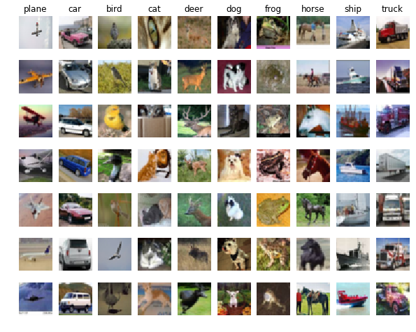
# Visualize some examples from the dataset.
# We show a few examples of training images from each class.
classes = ['plane', 'car', 'bird', 'cat', 'deer', 'dog', 'frog', 'horse', 'ship', 'truck']
num_classes = len(classes)
samples_per_class = 7
for y, cls in enumerate(classes):
    idxs = np.flatnonzero(y_train == y)
    idxs = np.random.choice(idxs, samples_per_class, replace=False)
    for i, idx in enumerate(idxs):
        plt_idx = i * num_classes + y + 1
        plt.subplot(samples_per_class, num_classes, plt_idx)
        plt.imshow(X_train[idx].astype('uint8'))
        plt.axis('off')
        if i == 0:
            plt.title(cls)
plt.show()
# Split the data into train, val, and test sets. In addition we will
# create a small development set as a subset of the training data;
# we can use this for development so our code runs faster.
num_training = 49000
num_validation = 1000
num_test = 1000
num_dev = 500

# Our validation set will be num_validation points from the original
# training set.
mask = range(num_training, num_training + num_validation)
X_val = X_train[mask]
y_val = y_train[mask]

# Our training set will be the first num_train points from the original
# training set.
mask = range(num_training)
X_train = X_train[mask]
y_train = y_train[mask]

# We will also make a development set, which is a small subset of
# the training set.
mask = np.random.choice(num_training, num_dev, replace=False)
X_dev = X_train[mask]
y_dev = y_train[mask]

# We use the first num_test points of the original test set as our
# test set.
mask = range(num_test)
X_test = X_test[mask]
y_test = y_test[mask]

print('Train data shape: ', X_train.shape)
print('Train labels shape: ', y_train.shape)
print('Validation data shape: ', X_val.shape)
print('Validation labels shape: ', y_val.shape)
print('Test data shape: ', X_test.shape)
print('Test labels shape: ', y_test.shape)
Train data shape:  (49000, 32, 32, 3)
Train labels shape:  (49000,)
Validation data shape:  (1000, 32, 32, 3)
Validation labels shape:  (1000,)
Test data shape:  (1000, 32, 32, 3)
Test labels shape:  (1000,)
# Preprocessing: reshape the image data into rows
X_train = np.reshape(X_train, (X_train.shape[0], -1))
X_val = np.reshape(X_val, (X_val.shape[0], -1))
X_test = np.reshape(X_test, (X_test.shape[0], -1))
X_dev = np.reshape(X_dev, (X_dev.shape[0], -1))

# As a sanity check, print out the shapes of the data
print('Training data shape: ', X_train.shape)
print('Validation data shape: ', X_val.shape)
print('Test data shape: ', X_test.shape)
print('dev data shape: ', X_dev.shape)
Training data shape:  (49000, 3072)
Validation data shape:  (1000, 3072)
Test data shape:  (1000, 3072)
dev data shape:  (500, 3072)
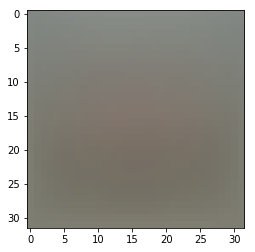
# Preprocessing: subtract the mean image
# first: compute the image mean based on the training data
mean_image = np.mean(X_train, axis=0)
print(mean_image[:10]) # print a few of the elements
plt.figure(figsize=(4,4))
plt.imshow(mean_image.reshape((32,32,3)).astype('uint8')) # visualize the mean image
plt.show()

# second: subtract the mean image from train and test data
X_train -= mean_image
X_val -= mean_image
X_test -= mean_image
X_dev -= mean_image

# third: append the bias dimension of ones (i.e. bias trick) so that our SVM
# only has to worry about optimizing a single weight matrix W.
X_train = np.hstack([X_train, np.ones((X_train.shape[0], 1))])
X_val = np.hstack([X_val, np.ones((X_val.shape[0], 1))])
X_test = np.hstack([X_test, np.ones((X_test.shape[0], 1))])
X_dev = np.hstack([X_dev, np.ones((X_dev.shape[0], 1))])

print(X_train.shape, X_val.shape, X_test.shape, X_dev.shape)
[130.64189796 135.98173469 132.47391837 130.05569388 135.34804082
 131.75402041 130.96055102 136.14328571 132.47636735 131.48467347]
(49000, 3073) (1000, 3073) (1000, 3073) (500, 3073)
SVM Classifier
Your code for this section will all be written inside cs231n/classifiers/linear_svm.py.
As you can see, we have prefilled the function compute_loss_naive which uses for loops to evaluate the multiclass SVM loss function.
# Evaluate the naive implementation of the loss we provided for you:
from cs231n.classifiers.linear_svm import svm_loss_naive
import time

# generate a random SVM weight matrix of small numbers
W = np.random.randn(3073, 10) * 0.0001


loss, grad = svm_loss_naive(W, X_dev, y_dev, 0.000005)
print('loss: %f' % (loss, ))
#print('Gradient of Loss Function with respect to W: %', grad)
loss: 9.009948
The grad returned from the function above is right now all zero. Derive and implement the gradient for the SVM cost function and implement it inline inside the function svm_loss_naive. You will find it helpful to interleave your new code inside the existing function.
To check that you have correctly implemented the gradient correctly, you can numerically estimate the gradient of the loss function and compare the numeric estimate to the gradient that you computed. We have provided code that does this for you:
# Once you've implemented the gradient, recompute it with the code below
# and gradient check it with the function we provided for you

# Compute the loss and its gradient at W.
loss, grad = svm_loss_naive(W, X_dev, y_dev, 0.0)

# Numerically compute the gradient along several randomly chosen dimensions, and
# compare them with your analytically computed gradient. The numbers should match
# almost exactly along all dimensions.
from cs231n.gradient_check import grad_check_sparse
f = lambda w: svm_loss_naive(w, X_dev, y_dev, 0.0)[0]
grad_numerical = grad_check_sparse(f, W, grad)

# do the gradient check once again with regularization turned on
# you didn't forget the regularization gradient did you?
loss, grad = svm_loss_naive(W, X_dev, y_dev, 5e1)
f = lambda w: svm_loss_naive(w, X_dev, y_dev, 5e1)[0]
grad_numerical = grad_check_sparse(f, W, grad)
numerical: -1.427635 analytic: -1.497210, relative error: 2.378780e-02
numerical: 0.629017 analytic: 0.552066, relative error: 6.515333e-02
numerical: -4.783666 analytic: -4.836789, relative error: 5.521883e-03
numerical: -2.737096 analytic: -2.737096, relative error: 8.094983e-11
numerical: -35.135378 analytic: -35.133947, relative error: 2.036525e-05
numerical: 16.193813 analytic: 16.242888, relative error: 1.512972e-03
numerical: 2.117024 analytic: 2.117024, relative error: 5.781809e-11
numerical: -4.754289 analytic: -4.754289, relative error: 3.975646e-11
numerical: -34.942481 analytic: -34.937043, relative error: 7.783062e-05
numerical: 3.911415 analytic: 3.911415, relative error: 2.960998e-11
numerical: -17.359753 analytic: -17.360248, relative error: 1.424986e-05
numerical: 13.603556 analytic: 13.605670, relative error: 7.771505e-05
numerical: -6.239910 analytic: -6.271963, relative error: 2.561834e-03
numerical: -18.608776 analytic: -18.598920, relative error: 2.648993e-04
numerical: 18.581689 analytic: 18.579512, relative error: 5.860116e-05
numerical: 21.625559 analytic: 21.627082, relative error: 3.522931e-05
numerical: 23.269252 analytic: 23.270786, relative error: 3.295696e-05
numerical: 20.114998 analytic: 20.117100, relative error: 5.225250e-05
numerical: 15.177704 analytic: 15.238198, relative error: 1.988899e-03
numerical: -4.839053 analytic: -4.845355, relative error: 6.507791e-04
# Next implement the function svm_loss_vectorized; for now only compute the loss;
# we will implement the gradient in a moment.
tic = time.time()
loss_naive, grad_naive = svm_loss_naive(W, X_dev, y_dev, 0.000005)
toc = time.time()
print('Naive loss: %e computed in %fs' % (loss_naive, toc - tic))

from cs231n.classifiers.linear_svm import svm_loss_vectorized
tic = time.time()
loss_vectorized, _ = svm_loss_vectorized(W, X_dev, y_dev, 0.000005)
toc = time.time()
print('Vectorized loss: %e computed in %fs' % (loss_vectorized, toc - tic))

# The losses should match but your vectorized implementation should be much faster.
print('difference: %f' % (loss_naive - loss_vectorized))
Naive loss: 9.009948e+00 computed in 0.197585s
Vectorized loss: 9.009948e+00 computed in 0.020286s
difference: 0.000000
# Complete the implementation of svm_loss_vectorized, and compute the gradient
# of the loss function in a vectorized way.

# The naive implementation and the vectorized implementation should match, but
# the vectorized version should still be much faster.
tic = time.time()
_, grad_naive = svm_loss_naive(W, X_dev, y_dev, 0.000005)
toc = time.time()
print('Naive loss and gradient: computed in %fs' % (toc - tic))

tic = time.time()
_, grad_vectorized = svm_loss_vectorized(W, X_dev, y_dev, 0.000005)
toc = time.time()
print('Vectorized loss and gradient: computed in %fs' % (toc - tic))

# The loss is a single number, so it is easy to compare the values computed
# by the two implementations. The gradient on the other hand is a matrix, so
# we use the Frobenius norm to compare them.
difference = np.linalg.norm(grad_naive - grad_vectorized, ord='fro')
print('difference: %f' % difference)
Naive loss and gradient: computed in 0.195149s
Vectorized loss and gradient: computed in 0.004495s
difference: 0.000000
Stochastic Gradient Descent
We now have vectorized and efficient expressions for the loss, the gradient and our gradient matches the numerical gradient. We are therefore ready to do SGD to minimize the loss.
# In the file linear_classifier.py, implement SGD in the function
# LinearClassifier.train() and then run it with the code below.
from cs231n.classifiers import LinearSVM
svm = LinearSVM()
tic = time.time()
loss_hist = svm.train(X_train, y_train, learning_rate=1e-7, reg=2.5e4,
                      num_iters=1500, batch_size=200, verbose=True)
toc = time.time()
print('That took %fs' % (toc - tic))
iteration 0 / 1500: loss 400.177696
iteration 100 / 1500: loss 239.166708
iteration 200 / 1500: loss 145.709877
iteration 300 / 1500: loss 89.749298
iteration 400 / 1500: loss 55.983948
iteration 500 / 1500: loss 35.882957
iteration 600 / 1500: loss 23.684348
iteration 700 / 1500: loss 16.331219
iteration 800 / 1500: loss 12.441470
iteration 900 / 1500: loss 8.510883
iteration 1000 / 1500: loss 7.446843
iteration 1100 / 1500: loss 6.540311
iteration 1200 / 1500: loss 5.422131
iteration 1300 / 1500: loss 5.788476
iteration 1400 / 1500: loss 5.631743
That took 11.900724s
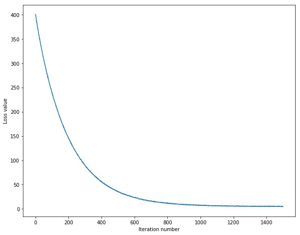
# A useful debugging strategy is to plot the loss as a function of
# iteration number:
plt.plot(loss_hist)
plt.xlabel('Iteration number')
plt.ylabel('Loss value')
plt.show()
# Write the LinearSVM.predict function and evaluate the performance on both the
# training and validation set
y_train_pred = svm.predict(X_train)
print('training accuracy: %f' % (np.mean(y_train == y_train_pred), ))
y_val_pred = svm.predict(X_val)
print('validation accuracy: %f' % (np.mean(y_val == y_val_pred), ))
training accuracy: 0.381224
validation accuracy: 0.379000
# Use the validation set to tune hyperparameters (regularization strength and
# learning rate). You should experiment with different ranges for the learning
# rates and regularization strengths; if you are careful you should be able to
# get a classification accuracy of about 0.39 on the validation set.

#Note: you may see runtime/overflow warnings during hyper-parameter search.
# This may be caused by extreme values, and is not a bug.

learning_rates = [1e-8, 1e-7, 2e-7]
regularization_strengths = [1e4, 2e4, 3e4, 4e4, 5e4, 6e4, 7e4, 8e4, 1e5]

# results is dictionary mapping tuples of the form
# (learning_rate, regularization_strength) to tuples of the form
# (training_accuracy, validation_accuracy). The accuracy is simply the fraction
# of data points that are correctly classified.
results = {}
best_val = -1   # The highest validation accuracy that we have seen so far.
best_svm = None # The LinearSVM object that achieved the highest validation rate.

################################################################################
# TODO:                                                                        #
# Write code that chooses the best hyperparameters by tuning on the validation #
# set. For each combination of hyperparameters, train a linear SVM on the      #
# training set, compute its accuracy on the training and validation sets, and  #
# store these numbers in the results dictionary. In addition, store the best   #
# validation accuracy in best_val and the LinearSVM object that achieves this  #
# accuracy in best_svm.                                                        #
#                                                                              #
# Hint: You should use a small value for num_iters as you develop your         #
# validation code so that the SVMs don't take much time to train; once you are #
# confident that your validation code works, you should rerun the validation   #
# code with a larger value for num_iters.                                      #
################################################################################
# *****START OF YOUR CODE (DO NOT DELETE/MODIFY THIS LINE)*****

for l in learning_rates:
    for r in regularization_strengths:
        svm = LinearSVM()
        svm.train(X_train, y_train, learning_rate=l, reg=r, num_iters=1500, batch_size=200)
        y_train_pred = svm.predict(X_train)
        y_val_pred = svm.predict(X_val)
        training_accuracy = np.mean(y_train == y_train_pred)
        validation_accuracy = np.mean(y_val == y_val_pred)
        results[(l, r)] = (training_accuracy, validation_accuracy)
        if validation_accuracy > best_val:
            best_val = validation_accuracy
            best_svm = svm

# *****END OF YOUR CODE (DO NOT DELETE/MODIFY THIS LINE)*****

# Print out results.
for lr, reg in sorted(results):
    train_accuracy, val_accuracy = results[(lr, reg)]
    print('lr %e reg %e train accuracy: %f val accuracy: %f' % (
                lr, reg, train_accuracy, val_accuracy))

print('best validation accuracy achieved during cross-validation: %f' % best_val)
lr 1.000000e-08 reg 1.000000e+04 train accuracy: 0.217857 val accuracy: 0.224000
lr 1.000000e-08 reg 2.000000e+04 train accuracy: 0.232388 val accuracy: 0.240000
lr 1.000000e-08 reg 3.000000e+04 train accuracy: 0.241490 val accuracy: 0.238000
lr 1.000000e-08 reg 4.000000e+04 train accuracy: 0.245286 val accuracy: 0.260000
lr 1.000000e-08 reg 5.000000e+04 train accuracy: 0.247714 val accuracy: 0.256000
lr 1.000000e-08 reg 6.000000e+04 train accuracy: 0.259571 val accuracy: 0.252000
lr 1.000000e-08 reg 7.000000e+04 train accuracy: 0.264898 val accuracy: 0.294000
lr 1.000000e-08 reg 8.000000e+04 train accuracy: 0.281082 val accuracy: 0.308000
lr 1.000000e-08 reg 1.000000e+05 train accuracy: 0.307102 val accuracy: 0.314000
lr 1.000000e-07 reg 1.000000e+04 train accuracy: 0.374531 val accuracy: 0.370000
lr 1.000000e-07 reg 2.000000e+04 train accuracy: 0.384673 val accuracy: 0.383000
lr 1.000000e-07 reg 3.000000e+04 train accuracy: 0.380224 val accuracy: 0.385000
lr 1.000000e-07 reg 4.000000e+04 train accuracy: 0.374163 val accuracy: 0.381000
lr 1.000000e-07 reg 5.000000e+04 train accuracy: 0.370714 val accuracy: 0.389000
lr 1.000000e-07 reg 6.000000e+04 train accuracy: 0.364571 val accuracy: 0.379000
lr 1.000000e-07 reg 7.000000e+04 train accuracy: 0.365204 val accuracy: 0.365000
lr 1.000000e-07 reg 8.000000e+04 train accuracy: 0.354367 val accuracy: 0.366000
lr 1.000000e-07 reg 1.000000e+05 train accuracy: 0.358224 val accuracy: 0.364000
lr 2.000000e-07 reg 1.000000e+04 train accuracy: 0.381102 val accuracy: 0.363000
lr 2.000000e-07 reg 2.000000e+04 train accuracy: 0.377531 val accuracy: 0.378000
lr 2.000000e-07 reg 3.000000e+04 train accuracy: 0.372265 val accuracy: 0.375000
lr 2.000000e-07 reg 4.000000e+04 train accuracy: 0.358224 val accuracy: 0.368000
lr 2.000000e-07 reg 5.000000e+04 train accuracy: 0.365980 val accuracy: 0.367000
lr 2.000000e-07 reg 6.000000e+04 train accuracy: 0.352714 val accuracy: 0.363000
lr 2.000000e-07 reg 7.000000e+04 train accuracy: 0.350612 val accuracy: 0.356000
lr 2.000000e-07 reg 8.000000e+04 train accuracy: 0.350694 val accuracy: 0.356000
lr 2.000000e-07 reg 1.000000e+05 train accuracy: 0.343633 val accuracy: 0.368000
best validation accuracy achieved during cross-validation: 0.389000
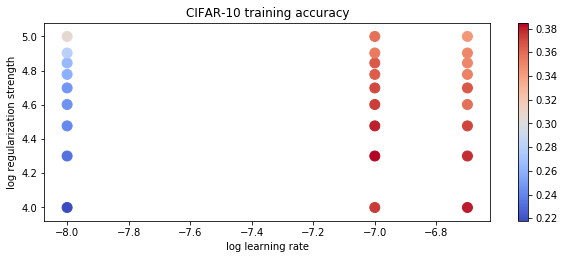
# Visualize the cross-validation results
import math
x_scatter = [math.log10(x[0]) for x in results]
y_scatter = [math.log10(x[1]) for x in results]

# plot training accuracy
marker_size = 100
colors = [results[x][0] for x in results]
plt.subplot(2, 1, 1)
plt.scatter(x_scatter, y_scatter, marker_size, c=colors, cmap=plt.cm.coolwarm)
plt.colorbar()
plt.xlabel('log learning rate')
plt.ylabel('log regularization strength')
plt.title('CIFAR-10 training accuracy')
Text(0.5,1,'CIFAR-10 training accuracy')
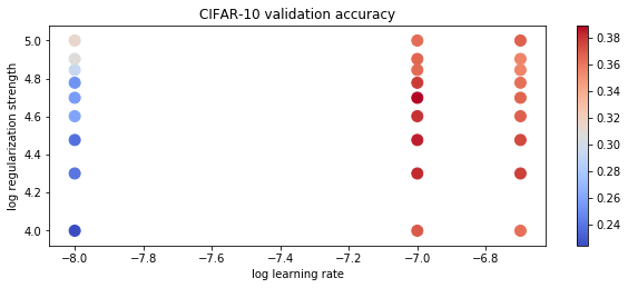
# plot validation accuracy
colors = [results[x][1] for x in results] # default size of markers is 20
plt.subplot(2, 1, 2)
plt.scatter(x_scatter, y_scatter, marker_size, c=colors, cmap=plt.cm.coolwarm)
plt.colorbar()
plt.xlabel('log learning rate')
plt.ylabel('log regularization strength')
plt.title('CIFAR-10 validation accuracy')
plt.show()
# Evaluate the best svm on test set
y_test_pred = best_svm.predict(X_test)
test_accuracy = np.mean(y_test == y_test_pred)
print('linear SVM on raw pixels final test set accuracy: %f' % test_accuracy)
linear SVM on raw pixels final test set accuracy: 0.350000
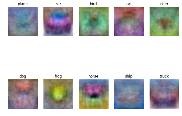
# Visualize the learned weights for each class.
# Depending on your choice of learning rate and regularization strength, these may
# or may not be nice to look at.
w = best_svm.W[:-1,:] # strip out the bias
w = w.reshape(32, 32, 3, 10)
w_min, w_max = np.min(w), np.max(w)
classes = ['plane', 'car', 'bird', 'cat', 'deer', 'dog', 'frog', 'horse', 'ship', 'truck']
for i in range(10):
    plt.subplot(2, 5, i + 1)

    # Rescale the weights to be between 0 and 255
    wimg = 255.0 * (w[:, :, :, i].squeeze() - w_min) / (w_max - w_min)
    plt.imshow(wimg.astype('uint8'))
    plt.axis('off')
    plt.title(classes[i])