Batch Normalization
Original source code and content provided by Stanford University, see course notes for cs231n: Convolutional Neural Networks for Visual Recognition.
Batch Normalization
One way to make deep networks easier to train is to use more sophisticated optimization procedures such as SGD+momentum, RMSProp, or Adam. Another strategy is to change the architecture of the network to make it easier to train. One idea along these lines is batch normalization which was proposed by [1] in 2015.
The idea is relatively straightforward. Machine learning methods tend to work better when their input data consists of uncorrelated features with zero mean and unit variance. When training a neural network, we can preprocess the data before feeding it to the network to explicitly decorrelate its features; this will ensure that the first layer of the network sees data that follows a nice distribution. However, even if we preprocess the input data, the activations at deeper layers of the network will likely no longer be decorrelated and will no longer have zero mean or unit variance since they are output from earlier layers in the network. Even worse, during the training process the distribution of features at each layer of the network will shift as the weights of each layer are updated.
The authors of [1] hypothesize that the shifting distribution of features inside deep neural networks may make training deep networks more difficult. To overcome this problem, [1] proposes to insert batch normalization layers into the network. At training time, a batch normalization layer uses a minibatch of data to estimate the mean and standard deviation of each feature. These estimated means and standard deviations are then used to center and normalize the features of the minibatch. A running average of these means and standard deviations is kept during training, and at test time these running averages are used to center and normalize features.
It is possible that this normalization strategy could reduce the representational power of the network, since it may sometimes be optimal for certain layers to have features that are not zero-mean or unit variance. To this end, the batch normalization layer includes learnable shift and scale parameters for each feature dimension.
# As usual, a bit of setup
import time
import numpy as np
import matplotlib.pyplot as plt
from cs231n.classifiers.fc_net import *
from cs231n.data_utils import get_CIFAR10_data
from cs231n.gradient_check import eval_numerical_gradient, eval_numerical_gradient_array
from cs231n.solver import Solver

%matplotlib inline
plt.rcParams['figure.figsize'] = (10.0, 8.0) # set default size of plots
plt.rcParams['image.interpolation'] = 'nearest'
plt.rcParams['image.cmap'] = 'gray'

# for auto-reloading external modules
# see http://stackoverflow.com/questions/1907993/autoreload-of-modules-in-ipython
%load_ext autoreload
%autoreload 2

def rel_error(x, y):
    """ returns relative error """
    return np.max(np.abs(x - y) / (np.maximum(1e-8, np.abs(x) + np.abs(y))))

def print_mean_std(x,axis=0):
    print('  means: ', x.mean(axis=axis))
    print('  stds:  ', x.std(axis=axis))
    print()
The autoreload extension is already loaded. To reload it, use:
  %reload_ext autoreload
# Load the (preprocessed) CIFAR10 data.
data = get_CIFAR10_data()
for k, v in data.items():
  print('%s: ' % k, v.shape)
X_train:  (49000, 3, 32, 32)
y_train:  (49000,)
X_val:  (1000, 3, 32, 32)
y_val:  (1000,)
X_test:  (1000, 3, 32, 32)
y_test:  (1000,)
Batch normalization: forward
In the file cs231n/layers.py, implement the batch normalization forward pass in the function batchnorm_forward. Once you have done so, run the following to test your implementation.
Referencing the paper linked to above in [1] may be helpful!
# Check the training-time forward pass by checking means and variances
# of features both before and after batch normalization

# Simulate the forward pass for a two-layer network
np.random.seed(231)
N, D1, D2, D3 = 200, 50, 60, 3
X = np.random.randn(N, D1)
W1 = np.random.randn(D1, D2)
W2 = np.random.randn(D2, D3)
a = np.maximum(0, X.dot(W1)).dot(W2)

print('Before batch normalization:')
print_mean_std(a,axis=0)

gamma = np.ones((D3,))
beta = np.zeros((D3,))
# Means should be close to zero and stds close to one
print('After batch normalization (gamma=1, beta=0)')
a_norm, _ = batchnorm_forward(a, gamma, beta, {'mode': 'train'})
print_mean_std(a_norm,axis=0)

beta = np.asarray([11.0, 12.0, 13.0])
gamma = np.asarray([1.0, 2.0, 3.0])
# Now means should be close to beta and stds close to gamma
print('After batch normalization (gamma=', gamma, ', beta=', beta, ')')
a_norm, _ = batchnorm_forward(a, gamma, beta, {'mode': 'train'})
print_mean_std(a_norm,axis=0)
Before batch normalization:
  means:  [ -2.3814598  -13.18038246   1.91780462]
  stds:   [27.18502186 34.21455511 37.68611762]

After batch normalization (gamma=1, beta=0)
  means:  [2.22044605e-17 8.16013923e-17 4.57966998e-17]
  stds:   [0.99999999 1.         1.        ]

After batch normalization (gamma= [1. 2. 3.] , beta= [11. 12. 13.] )
  means:  [11. 12. 13.]
  stds:   [0.99999999 1.99999999 2.99999999]
# Check the test-time forward pass by running the training-time
# forward pass many times to warm up the running averages, and then
# checking the means and variances of activations after a test-time
# forward pass.

np.random.seed(231)
N, D1, D2, D3 = 200, 50, 60, 3
W1 = np.random.randn(D1, D2)
W2 = np.random.randn(D2, D3)

bn_param = {'mode': 'train'}
gamma = np.ones(D3)
beta = np.zeros(D3)

for t in range(50):
  X = np.random.randn(N, D1)
  a = np.maximum(0, X.dot(W1)).dot(W2)
  batchnorm_forward(a, gamma, beta, bn_param)

bn_param['mode'] = 'test'
X = np.random.randn(N, D1)
a = np.maximum(0, X.dot(W1)).dot(W2)
a_norm, _ = batchnorm_forward(a, gamma, beta, bn_param)

# Means should be close to zero and stds close to one, but will be
# noisier than training-time forward passes.
print('After batch normalization (test-time):')
print_mean_std(a_norm,axis=0)
After batch normalization (test-time):
  means:  [-0.03927354 -0.04349152 -0.10452688]
  stds:   [1.01531428 1.01238373 0.97819988]
Batch normalization: backward
Now implement the backward pass for batch normalization in the function batchnorm_backward.
To derive the backward pass you should write out the computation graph for batch normalization and backprop through each of the intermediate nodes. Some intermediates may have multiple outgoing branches; make sure to sum gradients across these branches in the backward pass.
Once you have finished, run the following to numerically check your backward pass.
# Gradient check batchnorm backward pass
np.random.seed(231)
N, D = 4, 5
x = 5 * np.random.randn(N, D) + 12
gamma = np.random.randn(D)
beta = np.random.randn(D)
dout = np.random.randn(N, D)

bn_param = {'mode': 'train'}
fx = lambda x: batchnorm_forward(x, gamma, beta, bn_param)[0]
fg = lambda a: batchnorm_forward(x, a, beta, bn_param)[0]
fb = lambda b: batchnorm_forward(x, gamma, b, bn_param)[0]

dx_num = eval_numerical_gradient_array(fx, x, dout)
da_num = eval_numerical_gradient_array(fg, gamma.copy(), dout)
db_num = eval_numerical_gradient_array(fb, beta.copy(), dout)

_, cache = batchnorm_forward(x, gamma, beta, bn_param)
dx, dgamma, dbeta = batchnorm_backward(dout, cache)
#You should expect to see relative errors between 1e-13 and 1e-8
print('dx error: ', rel_error(dx_num, dx))
print('dgamma error: ', rel_error(da_num, dgamma))
print('dbeta error: ', rel_error(db_num, dbeta))
dx error:  1.7029261167605239e-09
dgamma error:  7.420414216247087e-13
dbeta error:  2.8795057655839487e-12
Batch normalization: alternative backward
In class we talked about two different implementations for the sigmoid backward pass. One strategy is to write out a computation graph composed of simple operations and backprop through all intermediate values. Another strategy is to work out the derivatives on paper. For example, you can derive a very simple formula for the sigmoid function’s backward pass by simplifying gradients on paper.
Surprisingly, it turns out that you can do a similar simplification for the batch normalization backward pass too!
In the forward pass, given a set of inputs ,
we first calculate the mean $\mu$ and variance $v$. With $\mu$ and $v$ calculated, we can calculate the standard deviation $\sigma$ and normalized data $Y$. The equations and graph illustration below describe the computation ($y_i$ is the i-th element of the vector $Y$).
\begin{align}
& \mu=\frac{1}{N}\sum_{k=1}^N x_k & v=\frac{1}{N}\sum_{k=1}^N (x_k-\mu)^2
& \sigma=\sqrt{v+\epsilon} & y_i=\frac{x_i-\mu}{\sigma}
\end{align}
<img src=”/assets/png/notebook_images/batchnorm_graph.png” width=691 height=202>
The meat of our problem during backpropagation is to compute $\frac{\partial L}{\partial X}$, given the upstream gradient we receive, $\frac{\partial L}{\partial Y}.$ To do this, recall the chain rule in calculus gives us $\frac{\partial L}{\partial X} = \frac{\partial L}{\partial Y} \cdot \frac{\partial Y}{\partial X}$.
The unknown/hart part is $\frac{\partial Y}{\partial X}$. We can find this by first deriving step-by-step our local gradients at $\frac{\partial v}{\partial X}$, $\frac{\partial \mu}{\partial X}$, $\frac{\partial \sigma}{\partial v}$, $\frac{\partial Y}{\partial \sigma}$, and $\frac{\partial Y}{\partial \mu}$, and then use the chain rule to compose these gradients (which appear in the form of vectors!) appropriately to compute $\frac{\partial Y}{\partial X}$.
If it’s challenging to directly reason about the gradients over $X$ and $Y$ which require matrix multiplication, try reasoning about the gradients in terms of individual elements $x_i$ and $y_i$ first: in that case, you will need to come up with the derivations for $\frac{\partial L}{\partial x_i}$, by relying on the Chain Rule to first calculate the intermediate $\frac{\partial \mu}{\partial x_i}, \frac{\partial v}{\partial x_i}, \frac{\partial \sigma}{\partial x_i},$ then assemble these pieces to calculate $\frac{\partial y_i}{\partial x_i}$.
You should make sure each of the intermediary gradient derivations are all as simplified as possible, for ease of implementation.
After doing so, implement the simplified batch normalization backward pass in the function batchnorm_backward_alt and compare the two implementations by running the following. Your two implementations should compute nearly identical results, but the alternative implementation should be a bit faster.
np.random.seed(231)
N, D = 100, 500
x = 5 * np.random.randn(N, D) + 12
gamma = np.random.randn(D)
beta = np.random.randn(D)
dout = np.random.randn(N, D)

bn_param = {'mode': 'train'}
out, cache = batchnorm_forward(x, gamma, beta, bn_param)

t1 = time.time()
dx1, dgamma1, dbeta1 = batchnorm_backward(dout, cache)
t2 = time.time()
#dx2, dgamma2, dbeta2 = batchnorm_backward_alt(dout, cache)
#t3 = time.time()

#print('dx difference: ', rel_error(dx1, dx2))
#print('dgamma difference: ', rel_error(dgamma1, dgamma2))
#print('dbeta difference: ', rel_error(dbeta1, dbeta2))
#print('speedup: %.2fx' % ((t2 - t1) / (t3 - t2)))
Fully Connected Nets with Batch Normalization
Now that you have a working implementation for batch normalization, go back to your FullyConnectedNet in the file cs231n/classifiers/fc_net.py. Modify your implementation to add batch normalization.
Concretely, when the normalization flag is set to "batchnorm" in the constructor, you should insert a batch normalization layer before each ReLU nonlinearity. The outputs from the last layer of the network should not be normalized. Once you are done, run the following to gradient-check your implementation.
HINT: You might find it useful to define an additional helper layer similar to those in the file cs231n/layer_utils.py. If you decide to do so, do it in the file cs231n/classifiers/fc_net.py.
np.random.seed(231)
N, D, H1, H2, C = 2, 15, 20, 30, 10
X = np.random.randn(N, D)
y = np.random.randint(C, size=(N,))

# You should expect losses between 1e-4~1e-10 for W,
# losses between 1e-08~1e-10 for b,
# and losses between 1e-08~1e-09 for beta and gammas.
for reg in [0, 3.14]:
  print('Running check with reg = ', reg)
  model = FullyConnectedNet([H1, H2], input_dim=D, num_classes=C,
                            reg=reg, weight_scale=5e-2, dtype=np.float64,
                            normalization='batchnorm')

  loss, grads = model.loss(X, y)
  print('Initial loss: ', loss)

  for name in sorted(grads):
    f = lambda _: model.loss(X, y)[0]
    grad_num = eval_numerical_gradient(f, model.params[name], verbose=False, h=1e-5)
    print('%s relative error: %.2e' % (name, rel_error(grad_num, grads[name])))
  if reg == 0: print()
Running check with reg =  0
Initial loss:  2.3309802038647067
W1 relative error: 1.07e-05
W2 relative error: 3.91e-09
W3 relative error: 2.83e-07
b1 relative error: 4.67e-06
b2 relative error: 1.76e-09
b3 relative error: 1.40e-10

Running check with reg =  3.14
Initial loss:  62.00999987021252
W1 relative error: 2.85e-07
W2 relative error: 3.08e-07
W3 relative error: 1.53e-06
b1 relative error: 2.23e-03
b2 relative error: 6.49e-08
b3 relative error: 1.07e-09
Batchnorm for deep networks
Run the following to train a six-layer network on a subset of 1000 training examples both with and without batch normalization.
np.random.seed(231)
# Try training a very deep net with batchnorm
hidden_dims = [100, 100, 100, 100, 100]

data = get_CIFAR10_data()

num_train = 1000
small_data = {
  'X_train': data['X_train'][:num_train],
  'y_train': data['y_train'][:num_train],
  'X_val': data['X_val'],
  'y_val': data['y_val'],
}

for k, v in small_data.items():
  print('%s: ' % k, v.shape)

weight_scale = 2e-2
bn_model = FullyConnectedNet(hidden_dims, weight_scale=weight_scale, normalization='batchnorm')
model = FullyConnectedNet(hidden_dims, weight_scale=weight_scale, normalization=None)

print('Solver with batch norm:')
bn_solver = Solver(bn_model, small_data,
                num_epochs=10, batch_size=50,
                update_rule='adam',
                optim_config={
                  'learning_rate': 1e-3,
                },
                verbose=True,print_every=20)
bn_solver.train()

print('\nSolver without batch norm:')
solver = Solver(model, small_data,
                num_epochs=10, batch_size=50,
                update_rule='adam',
                optim_config={
                  'learning_rate': 1e-3,
                },
                verbose=True, print_every=20)
solver.train()
X_train:  (1000, 3, 32, 32)
y_train:  (1000,)
X_val:  (1000, 3, 32, 32)
y_val:  (1000,)
Solver with batch norm:
(Iteration 1 / 200) loss: 2.307831
(Epoch 0 / 10) train acc: 0.101000; val_acc: 0.106000
(Epoch 1 / 10) train acc: 0.284000; val_acc: 0.254000
(Iteration 21 / 200) loss: 1.969008
(Epoch 2 / 10) train acc: 0.385000; val_acc: 0.261000
(Iteration 41 / 200) loss: 2.106257
(Epoch 3 / 10) train acc: 0.424000; val_acc: 0.291000
(Iteration 61 / 200) loss: 1.749373
(Epoch 4 / 10) train acc: 0.470000; val_acc: 0.280000
(Iteration 81 / 200) loss: 1.397609
(Epoch 5 / 10) train acc: 0.532000; val_acc: 0.317000
(Iteration 101 / 200) loss: 1.359280
(Epoch 6 / 10) train acc: 0.608000; val_acc: 0.337000
(Iteration 121 / 200) loss: 1.177555
(Epoch 7 / 10) train acc: 0.679000; val_acc: 0.332000
(Iteration 141 / 200) loss: 1.225403
(Epoch 8 / 10) train acc: 0.736000; val_acc: 0.330000
(Iteration 161 / 200) loss: 0.748057
(Epoch 9 / 10) train acc: 0.771000; val_acc: 0.327000
(Iteration 181 / 200) loss: 0.802301
(Epoch 10 / 10) train acc: 0.772000; val_acc: 0.312000

Solver without batch norm:
(Iteration 1 / 200) loss: 2.302332
(Epoch 0 / 10) train acc: 0.129000; val_acc: 0.131000


C:\Users\abbottjc\Google Drive\School\UCD\Fall_2019\ELEC_5840_IndependentStudy\cs231_Stanford\spring1819_assignment2\cs231n\optim.py:163: RuntimeWarning: invalid value encountered in sqrt
  next_w += -(config['learning_rate'] * config['mt']) / (np.sqrt(config['vt']) + config['epsilon'])


(Epoch 1 / 10) train acc: 0.245000; val_acc: 0.212000
(Iteration 21 / 200) loss: 2.062543
(Epoch 2 / 10) train acc: 0.318000; val_acc: 0.270000
(Iteration 41 / 200) loss: 1.822040
(Epoch 3 / 10) train acc: 0.347000; val_acc: 0.262000
(Iteration 61 / 200) loss: 1.761721
(Epoch 4 / 10) train acc: 0.384000; val_acc: 0.286000
(Iteration 81 / 200) loss: 1.560298
(Epoch 5 / 10) train acc: 0.421000; val_acc: 0.295000
(Iteration 101 / 200) loss: 1.747118
(Epoch 6 / 10) train acc: 0.462000; val_acc: 0.307000
(Iteration 121 / 200) loss: 1.420507
(Epoch 7 / 10) train acc: 0.484000; val_acc: 0.295000
(Iteration 141 / 200) loss: 1.344577
(Epoch 8 / 10) train acc: 0.540000; val_acc: 0.317000
(Iteration 161 / 200) loss: 1.290093
(Epoch 9 / 10) train acc: 0.601000; val_acc: 0.333000
(Iteration 181 / 200) loss: 0.931621
(Epoch 10 / 10) train acc: 0.612000; val_acc: 0.320000
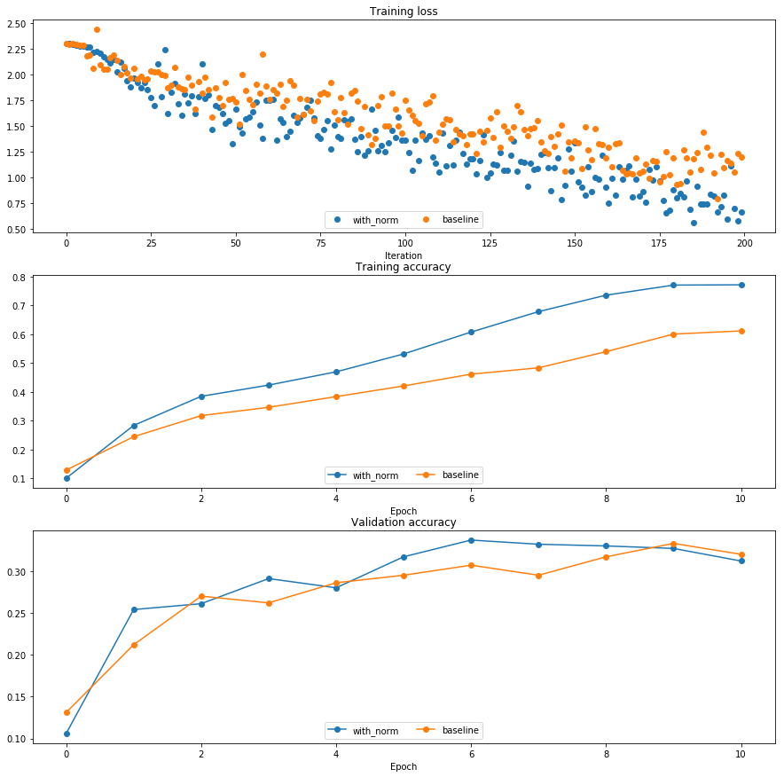
Run the following to visualize the results from two networks trained above. You should find that using batch normalization helps the network to converge much faster.
def plot_training_history(title, label, baseline, bn_solvers, plot_fn, bl_marker='.', bn_marker='.', labels=None):
    """utility function for plotting training history"""
    plt.title(title)
    plt.xlabel(label)
    bn_plots = [plot_fn(bn_solver) for bn_solver in bn_solvers]
    bl_plot = plot_fn(baseline)
    num_bn = len(bn_plots)
    for i in range(num_bn):
        label='with_norm'
        if labels is not None:
            label += str(labels[i])
        plt.plot(bn_plots[i], bn_marker, label=label)
    label='baseline'
    if labels is not None:
        label += str(labels[0])
    plt.plot(bl_plot, bl_marker, label=label)
    plt.legend(loc='lower center', ncol=num_bn+1)


plt.subplot(3, 1, 1)
plot_training_history('Training loss','Iteration', solver, [bn_solver], \
                      lambda x: x.loss_history, bl_marker='o', bn_marker='o')
plt.subplot(3, 1, 2)
plot_training_history('Training accuracy','Epoch', solver, [bn_solver], \
                      lambda x: x.train_acc_history, bl_marker='-o', bn_marker='-o')
plt.subplot(3, 1, 3)
plot_training_history('Validation accuracy','Epoch', solver, [bn_solver], \
                      lambda x: x.val_acc_history, bl_marker='-o', bn_marker='-o')

plt.gcf().set_size_inches(15, 15)
plt.show()
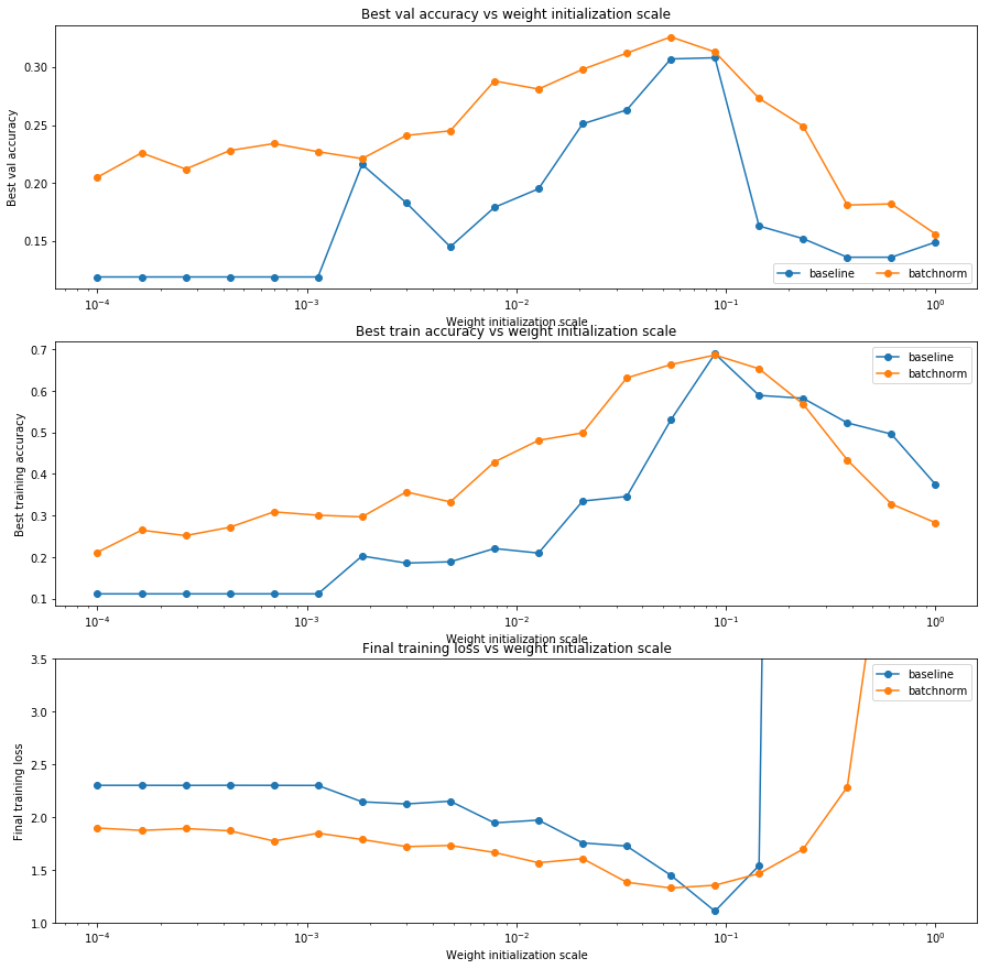
Batch normalization and initialization
We will now run a small experiment to study the interaction of batch normalization and weight initialization.
The first cell will train 8-layer networks both with and without batch normalization using different scales for weight initialization. The second layer will plot training accuracy, validation set accuracy, and training loss as a function of the weight initialization scale.
np.random.seed(231)
# Try training a very deep net with batchnorm
hidden_dims = [50, 50, 50, 50, 50, 50, 50]
num_train = 1000
small_data = {
  'X_train': data['X_train'][:num_train],
  'y_train': data['y_train'][:num_train],
  'X_val': data['X_val'],
  'y_val': data['y_val'],
}

bn_solvers_ws = {}
solvers_ws = {}
weight_scales = np.logspace(-4, 0, num=20)
for i, weight_scale in enumerate(weight_scales):
  print('Running weight scale %d / %d' % (i + 1, len(weight_scales)))
  bn_model = FullyConnectedNet(hidden_dims, weight_scale=weight_scale, normalization='batchnorm')
  model = FullyConnectedNet(hidden_dims, weight_scale=weight_scale, normalization=None)

  bn_solver = Solver(bn_model, small_data,
                  num_epochs=10, batch_size=50,
                  update_rule='adam',
                  optim_config={
                    'learning_rate': 1e-3,
                  },
                  verbose=False, print_every=200)
  bn_solver.train()
  bn_solvers_ws[weight_scale] = bn_solver

  solver = Solver(model, small_data,
                  num_epochs=10, batch_size=50,
                  update_rule='adam',
                  optim_config={
                    'learning_rate': 1e-3,
                  },
                  verbose=False, print_every=200)
  solver.train()
  solvers_ws[weight_scale] = solver
Running weight scale 1 / 20


C:\Users\abbottjc\Google Drive\School\UCD\Fall_2019\ELEC_5840_IndependentStudy\cs231_Stanford\spring1819_assignment2\cs231n\optim.py:163: RuntimeWarning: invalid value encountered in sqrt
  next_w += -(config['learning_rate'] * config['mt']) / (np.sqrt(config['vt']) + config['epsilon'])


Running weight scale 2 / 20
Running weight scale 3 / 20
Running weight scale 4 / 20
Running weight scale 5 / 20
Running weight scale 6 / 20
Running weight scale 7 / 20
Running weight scale 8 / 20
Running weight scale 9 / 20
Running weight scale 10 / 20
Running weight scale 11 / 20
Running weight scale 12 / 20
Running weight scale 13 / 20
Running weight scale 14 / 20
Running weight scale 15 / 20
Running weight scale 16 / 20
Running weight scale 17 / 20
Running weight scale 18 / 20
Running weight scale 19 / 20
Running weight scale 20 / 20
# Plot results of weight scale experiment
best_train_accs, bn_best_train_accs = [], []
best_val_accs, bn_best_val_accs = [], []
final_train_loss, bn_final_train_loss = [], []

for ws in weight_scales:
  best_train_accs.append(max(solvers_ws[ws].train_acc_history))
  bn_best_train_accs.append(max(bn_solvers_ws[ws].train_acc_history))

  best_val_accs.append(max(solvers_ws[ws].val_acc_history))
  bn_best_val_accs.append(max(bn_solvers_ws[ws].val_acc_history))

  final_train_loss.append(np.mean(solvers_ws[ws].loss_history[-100:]))
  bn_final_train_loss.append(np.mean(bn_solvers_ws[ws].loss_history[-100:]))

plt.subplot(3, 1, 1)
plt.title('Best val accuracy vs weight initialization scale')
plt.xlabel('Weight initialization scale')
plt.ylabel('Best val accuracy')
plt.semilogx(weight_scales, best_val_accs, '-o', label='baseline')
plt.semilogx(weight_scales, bn_best_val_accs, '-o', label='batchnorm')
plt.legend(ncol=2, loc='lower right')

plt.subplot(3, 1, 2)
plt.title('Best train accuracy vs weight initialization scale')
plt.xlabel('Weight initialization scale')
plt.ylabel('Best training accuracy')
plt.semilogx(weight_scales, best_train_accs, '-o', label='baseline')
plt.semilogx(weight_scales, bn_best_train_accs, '-o', label='batchnorm')
plt.legend()

plt.subplot(3, 1, 3)
plt.title('Final training loss vs weight initialization scale')
plt.xlabel('Weight initialization scale')
plt.ylabel('Final training loss')
plt.semilogx(weight_scales, final_train_loss, '-o', label='baseline')
plt.semilogx(weight_scales, bn_final_train_loss, '-o', label='batchnorm')
plt.legend()
plt.gca().set_ylim(1.0, 3.5)

plt.gcf().set_size_inches(15, 15)
plt.show()
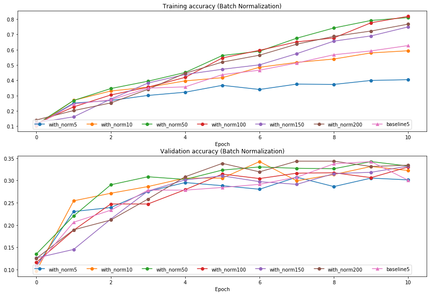
Batch normalization and batch size
We will now run a small experiment to study the interaction of batch normalization and batch size.
The first cell will train 6-layer networks both with and without batch normalization using different batch sizes. The second layer will plot training accuracy and validation set accuracy over time.
def run_batchsize_experiments(normalization_mode):
    np.random.seed(231)
    # Try training a very deep net with batchnorm
    hidden_dims = [100, 100, 100, 100, 100]
    num_train = 1000
    small_data = {
      'X_train': data['X_train'][:num_train],
      'y_train': data['y_train'][:num_train],
      'X_val': data['X_val'],
      'y_val': data['y_val'],
    }
    n_epochs=10
    weight_scale = 2e-2
    batch_sizes = [5,10,50,100,150,200]
    lr = 10**(-3.5)
    solver_bsize = batch_sizes[0]

    print('No normalization: batch size = ',solver_bsize)
    model = FullyConnectedNet(hidden_dims, weight_scale=weight_scale, normalization=None)
    solver = Solver(model, small_data,
                    num_epochs=n_epochs, batch_size=solver_bsize,
                    update_rule='adam',
                    optim_config={
                      'learning_rate': lr,
                    },
                    verbose=False)
    solver.train()

    bn_solvers = []
    for i in range(len(batch_sizes)):
        b_size=batch_sizes[i]
        print('Normalization: batch size = ',b_size)
        bn_model = FullyConnectedNet(hidden_dims, weight_scale=weight_scale, normalization=normalization_mode)
        bn_solver = Solver(bn_model, small_data,
                        num_epochs=n_epochs, batch_size=b_size,
                        update_rule='adam',
                        optim_config={
                          'learning_rate': lr,
                        },
                        verbose=False)
        bn_solver.train()
        bn_solvers.append(bn_solver)

    return bn_solvers, solver, batch_sizes

batch_sizes = [5,10,50]
bn_solvers_bsize, solver_bsize, batch_sizes = run_batchsize_experiments('batchnorm')
No normalization: batch size =  5


C:\Users\abbottjc\Google Drive\School\UCD\Fall_2019\ELEC_5840_IndependentStudy\cs231_Stanford\spring1819_assignment2\cs231n\optim.py:163: RuntimeWarning: invalid value encountered in sqrt
  next_w += -(config['learning_rate'] * config['mt']) / (np.sqrt(config['vt']) + config['epsilon'])


Normalization: batch size =  5
Normalization: batch size =  10
Normalization: batch size =  50
Normalization: batch size =  100
Normalization: batch size =  150
Normalization: batch size =  200
plt.subplot(2, 1, 1)
plot_training_history('Training accuracy (Batch Normalization)','Epoch', solver_bsize, bn_solvers_bsize, \
                      lambda x: x.train_acc_history, bl_marker='-^', bn_marker='-o', labels=batch_sizes)
plt.subplot(2, 1, 2)
plot_training_history('Validation accuracy (Batch Normalization)','Epoch', solver_bsize, bn_solvers_bsize, \
                      lambda x: x.val_acc_history, bl_marker='-^', bn_marker='-o', labels=batch_sizes)

plt.gcf().set_size_inches(15, 10)
plt.show()