PyTorch
Original source code and content provided by Stanford University, see course notes for cs231n: Convolutional Neural Networks for Visual Recognition.
What’s this PyTorch business?
You’ve written a lot of code in this assignment to provide a whole host of neural network functionality. Dropout, Batch Norm, and 2D convolutions are some of the workhorses of deep learning in computer vision. You’ve also worked hard to make your code efficient and vectorized.
For the last part of this assignment, though, we’re going to leave behind your beautiful codebase and instead migrate to one of two popular deep learning frameworks: in this instance, PyTorch (or TensorFlow, if you choose to use that notebook).
What is PyTorch?
PyTorch is a system for executing dynamic computational graphs over Tensor objects that behave similarly as numpy ndarray. It comes with a powerful automatic differentiation engine that removes the need for manual back-propagation.
Why?
- Our code will now run on GPUs! Much faster training. When using a framework like PyTorch or TensorFlow you can harness the power of the GPU for your own custom neural network architectures without having to write CUDA code directly (which is beyond the scope of this class).
- We want you to be ready to use one of these frameworks for your project so you can experiment more efficiently than if you were writing every feature you want to use by hand.
- We want you to stand on the shoulders of giants! TensorFlow and PyTorch are both excellent frameworks that will make your lives a lot easier, and now that you understand their guts, you are free to use them :)
- We want you to be exposed to the sort of deep learning code you might run into in academia or industry.
PyTorch versions
This notebook assumes that you are using PyTorch version 1.0. In some of the previous versions (e.g. before 0.4), Tensors had to be wrapped in Variable objects to be used in autograd; however Variables have now been deprecated. In addition 1.0 also separates a Tensor’s datatype from its device, and uses numpy-style factories for constructing Tensors rather than directly invoking Tensor constructors.
How will I learn PyTorch?
Justin Johnson has made an excellent tutorial for PyTorch.
You can also find the detailed API doc here. If you have other questions that are not addressed by the API docs, the PyTorch forum is a much better place to ask than StackOverflow.
Table of Contents
This assignment has 5 parts. You will learn PyTorch on three different levels of abstraction, which will help you understand it better and prepare you for the final project.
- Part I, Preparation: we will use CIFAR-10 dataset.
- Part II, Barebones PyTorch: Abstraction level 1, we will work directly with the lowest-level PyTorch Tensors.
- Part III, PyTorch Module API: Abstraction level 2, we will use
nn.Moduleto define arbitrary neural network architecture. - Part IV, PyTorch Sequential API: Abstraction level 3, we will use
nn.Sequentialto define a linear feed-forward network very conveniently. - Part V, CIFAR-10 open-ended challenge: please implement your own network to get as high accuracy as possible on CIFAR-10. You can experiment with any layer, optimizer, hyperparameters or other advanced features.
Here is a table of comparison:
| API | Flexibility | Convenience |
|---|---|---|
| Barebone | High | Low |
nn.Module |
High | Medium |
nn.Sequential |
Low | High |
Part I. Preparation
First, we load the CIFAR-10 dataset. This might take a couple minutes the first time you do it, but the files should stay cached after that.
In previous parts of the assignment we had to write our own code to download the CIFAR-10 dataset, preprocess it, and iterate through it in minibatches; PyTorch provides convenient tools to automate this process for us.
import torch
import torch.nn as nn
import torch.optim as optim
from torch.utils.data import DataLoader
from torch.utils.data import sampler

import torchvision.datasets as dset
import torchvision.transforms as T

import numpy as np
NUM_TRAIN = 49000

# The torchvision.transforms package provides tools for preprocessing data
# and for performing data augmentation; here we set up a transform to
# preprocess the data by subtracting the mean RGB value and dividing by the
# standard deviation of each RGB value; we've hardcoded the mean and std.
transform = T.Compose([
                T.ToTensor(),
                T.Normalize((0.4914, 0.4822, 0.4465), (0.2023, 0.1994, 0.2010))
            ])

# We set up a Dataset object for each split (train / val / test); Datasets load
# training examples one at a time, so we wrap each Dataset in a DataLoader which
# iterates through the Dataset and forms minibatches. We divide the CIFAR-10
# training set into train and val sets by passing a Sampler object to the
# DataLoader telling how it should sample from the underlying Dataset.
cifar10_train = dset.CIFAR10('./cs231n/datasets', train=True, download=True,
                             transform=transform)
loader_train = DataLoader(cifar10_train, batch_size=64,
                          sampler=sampler.SubsetRandomSampler(range(NUM_TRAIN)))

cifar10_val = dset.CIFAR10('./cs231n/datasets', train=True, download=True,
                           transform=transform)
loader_val = DataLoader(cifar10_val, batch_size=64,
                        sampler=sampler.SubsetRandomSampler(range(NUM_TRAIN, 50000)))

cifar10_test = dset.CIFAR10('./cs231n/datasets', train=False, download=True,
                            transform=transform)
loader_test = DataLoader(cifar10_test, batch_size=64)
Files already downloaded and verified
Files already downloaded and verified
Files already downloaded and verified
You have an option to use GPU by setting the flag to True below. It is not necessary to use GPU for this assignment. Note that if your computer does not have CUDA enabled, torch.cuda.is_available() will return False and this notebook will fallback to CPU mode.
The global variables dtype and device will control the data types throughout this assignment.
USE_GPU = True

dtype = torch.float32 # we will be using float throughout this tutorial

if USE_GPU and torch.cuda.is_available():
    device = torch.device('cuda')
else:
    device = torch.device('cpu')

# Constant to control how frequently we print train loss
print_every = 100

print('using device:', device)
using device: cuda
Part II. Barebones PyTorch
PyTorch ships with high-level APIs to help us define model architectures conveniently, which we will cover in Part II of this tutorial. In this section, we will start with the barebone PyTorch elements to understand the autograd engine better. After this exercise, you will come to appreciate the high-level model API more.
We will start with a simple fully-connected ReLU network with two hidden layers and no biases for CIFAR classification. This implementation computes the forward pass using operations on PyTorch Tensors, and uses PyTorch autograd to compute gradients. It is important that you understand every line, because you will write a harder version after the example.
When we create a PyTorch Tensor with requires_grad=True, then operations involving that Tensor will not just compute values; they will also build up a computational graph in the background, allowing us to easily backpropagate through the graph to compute gradients of some Tensors with respect to a downstream loss. Concretely if x is a Tensor with x.requires_grad == True then after backpropagation x.grad will be another Tensor holding the gradient of x with respect to the scalar loss at the end.
PyTorch Tensors: Flatten Function
A PyTorch Tensor is conceptionally similar to a numpy array: it is an n-dimensional grid of numbers, and like numpy PyTorch provides many functions to efficiently operate on Tensors. As a simple example, we provide a flatten function below which reshapes image data for use in a fully-connected neural network.
Recall that image data is typically stored in a Tensor of shape N x C x H x W, where:
- N is the number of datapoints
- C is the number of channels
- H is the height of the intermediate feature map in pixels
- W is the height of the intermediate feature map in pixels
This is the right way to represent the data when we are doing something like a 2D convolution, that needs spatial understanding of where the intermediate features are relative to each other. When we use fully connected affine layers to process the image, however, we want each datapoint to be represented by a single vector – it’s no longer useful to segregate the different channels, rows, and columns of the data. So, we use a “flatten” operation to collapse the C x H x W values per representation into a single long vector. The flatten function below first reads in the N, C, H, and W values from a given batch of data, and then returns a “view” of that data. “View” is analogous to numpy’s “reshape” method: it reshapes x’s dimensions to be N x ??, where ?? is allowed to be anything (in this case, it will be C x H x W, but we don’t need to specify that explicitly).
def flatten(x):
    N = x.shape[0] # read in N, C, H, W
    return x.view(N, -1)  # "flatten" the C * H * W values into a single vector per image

def test_flatten():
    x = torch.arange(12).view(2, 1, 3, 2)
    print('Before flattening: ', x)
    print('After flattening: ', flatten(x))

test_flatten()
Before flattening:  tensor([[[[ 0,  1],
          [ 2,  3],
          [ 4,  5]]],


        [[[ 6,  7],
          [ 8,  9],
          [10, 11]]]])
After flattening:  tensor([[ 0,  1,  2,  3,  4,  5],
        [ 6,  7,  8,  9, 10, 11]])
Barebones PyTorch: Two-Layer Network
Here we define a function two_layer_fc which performs the forward pass of a two-layer fully-connected ReLU network on a batch of image data. After defining the forward pass we check that it doesn’t crash and that it produces outputs of the right shape by running zeros through the network.
You don’t have to write any code here, but it’s important that you read and understand the implementation.
import torch.nn.functional as F  # useful stateless functions

def two_layer_fc(x, params):
    """
    A fully-connected neural networks; the architecture is:
    NN is fully connected -> ReLU -> fully connected layer.
    Note that this function only defines the forward pass;
    PyTorch will take care of the backward pass for us.

    The input to the network will be a minibatch of data, of shape
    (N, d1, ..., dM) where d1 * ... * dM = D. The hidden layer will have H units,
    and the output layer will produce scores for C classes.

    Inputs:
    - x: A PyTorch Tensor of shape (N, d1, ..., dM) giving a minibatch of
      input data.
    - params: A list [w1, w2] of PyTorch Tensors giving weights for the network;
      w1 has shape (D, H) and w2 has shape (H, C).

    Returns:
    - scores: A PyTorch Tensor of shape (N, C) giving classification scores for
      the input data x.
    """
    # first we flatten the image
    x = flatten(x)  # shape: [batch_size, C x H x W]

    w1, w2 = params

    # Forward pass: compute predicted y using operations on Tensors. Since w1 and
    # w2 have requires_grad=True, operations involving these Tensors will cause
    # PyTorch to build a computational graph, allowing automatic computation of
    # gradients. Since we are no longer implementing the backward pass by hand we
    # don't need to keep references to intermediate values.
    # you can also use `.clamp(min=0)`, equivalent to F.relu()
    x = F.relu(x.mm(w1))
    x = x.mm(w2)
    return x


def two_layer_fc_test():
    hidden_layer_size = 42
    x = torch.zeros((64, 50), dtype=dtype)  # minibatch size 64, feature dimension 50
    w1 = torch.zeros((50, hidden_layer_size), dtype=dtype)
    w2 = torch.zeros((hidden_layer_size, 10), dtype=dtype)
    scores = two_layer_fc(x, [w1, w2])
    print(scores.size())  # you should see [64, 10]

two_layer_fc_test()
torch.Size([64, 10])
Barebones PyTorch: Three-Layer ConvNet
Here you will complete the implementation of the function three_layer_convnet, which will perform the forward pass of a three-layer convolutional network. Like above, we can immediately test our implementation by passing zeros through the network. The network should have the following architecture:
- A convolutional layer (with bias) with
channel_1filters, each with shapeKW1 x KH1, and zero-padding of two - ReLU nonlinearity
- A convolutional layer (with bias) with
channel_2filters, each with shapeKW2 x KH2, and zero-padding of one - ReLU nonlinearity
- Fully-connected layer with bias, producing scores for C classes.
Note that we have no softmax activation here after our fully-connected layer: this is because PyTorch’s cross entropy loss performs a softmax activation for you, and by bundling that step in makes computation more efficient.
HINT: For convolutions: http://pytorch.org/docs/stable/nn.html#torch.nn.functional.conv2d; pay attention to the shapes of convolutional filters!
def three_layer_convnet(x, params):
    """
    Performs the forward pass of a three-layer convolutional network with the
    architecture defined above.

    Inputs:
    - x: A PyTorch Tensor of shape (N, 3, H, W) giving a minibatch of images
    - params: A list of PyTorch Tensors giving the weights and biases for the
      network; should contain the following:
      - conv_w1: PyTorch Tensor of shape (channel_1, 3, KH1, KW1) giving weights
        for the first convolutional layer
      - conv_b1: PyTorch Tensor of shape (channel_1,) giving biases for the first
        convolutional layer
      - conv_w2: PyTorch Tensor of shape (channel_2, channel_1, KH2, KW2) giving
        weights for the second convolutional layer
      - conv_b2: PyTorch Tensor of shape (channel_2,) giving biases for the second
        convolutional layer
      - fc_w: PyTorch Tensor giving weights for the fully-connected layer. Can you
        figure out what the shape should be?
      - fc_b: PyTorch Tensor giving biases for the fully-connected layer. Can you
        figure out what the shape should be?

    Returns:
    - scores: PyTorch Tensor of shape (N, C) giving classification scores for x
    """
    conv_w1, conv_b1, conv_w2, conv_b2, fc_w, fc_b = params
    scores = None
    ################################################################################
    # TODO: Implement the forward pass for the three-layer ConvNet.                #
    ################################################################################
    # *****START OF YOUR CODE (DO NOT DELETE/MODIFY THIS LINE)*****

    conv1_output = F.relu(F.conv2d(x, conv_w1, conv_b1, padding = 2))
    conv2_output = F.relu(F.conv2d(conv1_output, conv_w2, conv_b2, padding = 1))
    scores = flatten(conv2_output).mm(fc_w) + fc_b

    # *****END OF YOUR CODE (DO NOT DELETE/MODIFY THIS LINE)*****
    ################################################################################
    #                                 END OF YOUR CODE                             #
    ################################################################################
    return scores
After defining the forward pass of the ConvNet above, run the following cell to test your implementation.
When you run this function, scores should have shape (64, 10).
def three_layer_convnet_test():
    x = torch.zeros((64, 3, 32, 32), dtype=dtype)  # minibatch size 64, image size [3, 32, 32]

    conv_w1 = torch.zeros((6, 3, 5, 5), dtype=dtype)  # [out_channel, in_channel, kernel_H, kernel_W]
    conv_b1 = torch.zeros((6,))  # out_channel
    conv_w2 = torch.zeros((9, 6, 3, 3), dtype=dtype)  # [out_channel, in_channel, kernel_H, kernel_W]
    conv_b2 = torch.zeros((9,))  # out_channel

    # you must calculate the shape of the tensor after two conv layers, before the fully-connected layer
    fc_w = torch.zeros((9 * 32 * 32, 10))
    fc_b = torch.zeros(10)

    scores = three_layer_convnet(x, [conv_w1, conv_b1, conv_w2, conv_b2, fc_w, fc_b])
    print(scores.size())  # you should see [64, 10]
three_layer_convnet_test()
torch.Size([64, 10])
Barebones PyTorch: Initialization
Let’s write a couple utility methods to initialize the weight matrices for our models.
random_weight(shape)initializes a weight tensor with the Kaiming normalization method.zero_weight(shape)initializes a weight tensor with all zeros. Useful for instantiating bias parameters.
The random_weight function uses the Kaiming normal initialization method, described in:
He et al, Delving Deep into Rectifiers: Surpassing Human-Level Performance on ImageNet Classification, ICCV 2015, https://arxiv.org/abs/1502.01852
def random_weight(shape):
    """
    Create random Tensors for weights; setting requires_grad=True means that we
    want to compute gradients for these Tensors during the backward pass.
    We use Kaiming normalization: sqrt(2 / fan_in)
    """
    if len(shape) == 2:  # FC weight
        fan_in = shape[0]
    else:
        fan_in = np.prod(shape[1:]) # conv weight [out_channel, in_channel, kH, kW]
    # randn is standard normal distribution generator.
    w = torch.randn(shape, device=device, dtype=dtype) * np.sqrt(2. / fan_in)
    w.requires_grad = True
    return w

def zero_weight(shape):
    return torch.zeros(shape, device=device, dtype=dtype, requires_grad=True)

# create a weight of shape [3 x 5]
# you should see the type `torch.cuda.FloatTensor` if you use GPU.
# Otherwise it should be `torch.FloatTensor`
print(random_weight((3, 5)))
print(zero_weight(6))
tensor([[-1.2039, -0.0978,  1.2195, -0.5203,  0.7726],
        [-0.2437, -0.0190, -0.6214,  0.4438,  1.6301],
        [-0.7148, -0.3369,  1.0572, -0.8350, -0.2452]], device='cuda:0',
       requires_grad=True)
tensor([0., 0., 0., 0., 0., 0.], device='cuda:0', requires_grad=True)
Barebones PyTorch: Check Accuracy
When training the model we will use the following function to check the accuracy of our model on the training or validation sets.
When checking accuracy we don’t need to compute any gradients; as a result we don’t need PyTorch to build a computational graph for us when we compute scores. To prevent a graph from being built we scope our computation under a torch.no_grad() context manager.
def check_accuracy_part2(loader, model_fn, params):
    """
    Check the accuracy of a classification model.

    Inputs:
    - loader: A DataLoader for the data split we want to check
    - model_fn: A function that performs the forward pass of the model,
      with the signature scores = model_fn(x, params)
    - params: List of PyTorch Tensors giving parameters of the model

    Returns: Nothing, but prints the accuracy of the model
    """
    split = 'val' if loader.dataset.train else 'test'
    print('Checking accuracy on the %s set' % split)
    num_correct, num_samples = 0, 0
    with torch.no_grad():
        for x, y in loader:
            x = x.to(device=device, dtype=dtype)  # move to device, e.g. GPU
            y = y.to(device=device, dtype=torch.int64)
            scores = model_fn(x, params)
            _, preds = scores.max(1)
            num_correct += (preds == y).sum()
            num_samples += preds.size(0)
        acc = float(num_correct) / num_samples
        print('Got %d / %d correct (%.2f%%)' % (num_correct, num_samples, 100 * acc))
BareBones PyTorch: Training Loop
We can now set up a basic training loop to train our network. We will train the model using stochastic gradient descent without momentum. We will use torch.functional.cross_entropy to compute the loss; you can read about it here.
The training loop takes as input the neural network function, a list of initialized parameters ([w1, w2] in our example), and learning rate.
def train_part2(model_fn, params, learning_rate):
    """
    Train a model on CIFAR-10.

    Inputs:
    - model_fn: A Python function that performs the forward pass of the model.
      It should have the signature scores = model_fn(x, params) where x is a
      PyTorch Tensor of image data, params is a list of PyTorch Tensors giving
      model weights, and scores is a PyTorch Tensor of shape (N, C) giving
      scores for the elements in x.
    - params: List of PyTorch Tensors giving weights for the model
    - learning_rate: Python scalar giving the learning rate to use for SGD

    Returns: Nothing
    """
    for t, (x, y) in enumerate(loader_train):
        # Move the data to the proper device (GPU or CPU)
        x = x.to(device=device, dtype=dtype)
        y = y.to(device=device, dtype=torch.long)

        # Forward pass: compute scores and loss
        scores = model_fn(x, params)
        loss = F.cross_entropy(scores, y)

        # Backward pass: PyTorch figures out which Tensors in the computational
        # graph has requires_grad=True and uses backpropagation to compute the
        # gradient of the loss with respect to these Tensors, and stores the
        # gradients in the .grad attribute of each Tensor.
        loss.backward()

        # Update parameters. We don't want to backpropagate through the
        # parameter updates, so we scope the updates under a torch.no_grad()
        # context manager to prevent a computational graph from being built.
        with torch.no_grad():
            for w in params:
                w -= learning_rate * w.grad

                # Manually zero the gradients after running the backward pass
                w.grad.zero_()

        if t % print_every == 0:
            print('Iteration %d, loss = %.4f' % (t, loss.item()))
            check_accuracy_part2(loader_val, model_fn, params)
            print()
BareBones PyTorch: Train a Two-Layer Network
Now we are ready to run the training loop. We need to explicitly allocate tensors for the fully connected weights, w1 and w2.
Each minibatch of CIFAR has 64 examples, so the tensor shape is [64, 3, 32, 32].
After flattening, x shape should be [64, 3 * 32 * 32]. This will be the size of the first dimension of w1.
The second dimension of w1 is the hidden layer size, which will also be the first dimension of w2.
Finally, the output of the network is a 10-dimensional vector that represents the probability distribution over 10 classes.
You don’t need to tune any hyperparameters but you should see accuracies above 40% after training for one epoch.
hidden_layer_size = 4000
learning_rate = 1e-2

w1 = random_weight((3 * 32 * 32, hidden_layer_size))
w2 = random_weight((hidden_layer_size, 10))


train_part2(two_layer_fc, [w1, w2], learning_rate)
Iteration 0, loss = 3.2337
Checking accuracy on the val set
Got 120 / 1000 correct (12.00%)

Iteration 100, loss = 2.3173
Checking accuracy on the val set
Got 354 / 1000 correct (35.40%)

Iteration 200, loss = 1.8998
Checking accuracy on the val set
Got 409 / 1000 correct (40.90%)

Iteration 300, loss = 2.0188
Checking accuracy on the val set
Got 392 / 1000 correct (39.20%)

Iteration 400, loss = 1.9150
Checking accuracy on the val set
Got 416 / 1000 correct (41.60%)

Iteration 500, loss = 1.9243
Checking accuracy on the val set
Got 393 / 1000 correct (39.30%)

Iteration 600, loss = 1.5874
Checking accuracy on the val set
Got 451 / 1000 correct (45.10%)

Iteration 700, loss = 1.6174
Checking accuracy on the val set
Got 446 / 1000 correct (44.60%)
BareBones PyTorch: Training a ConvNet
In the below you should use the functions defined above to train a three-layer convolutional network on CIFAR. The network should have the following architecture:
- Convolutional layer (with bias) with 32 5x5 filters, with zero-padding of 2
- ReLU
- Convolutional layer (with bias) with 16 3x3 filters, with zero-padding of 1
- ReLU
- Fully-connected layer (with bias) to compute scores for 10 classes
You should initialize your weight matrices using the random_weight function defined above, and you should initialize your bias vectors using the zero_weight function above.
You don’t need to tune any hyperparameters, but if everything works correctly you should achieve an accuracy above 42% after one epoch.
learning_rate = 3e-3

channel_1 = 32
channel_2 = 16

conv_w1 = None
conv_b1 = None
conv_w2 = None
conv_b2 = None
fc_w = None
fc_b = None

################################################################################
# TODO: Initialize the parameters of a three-layer ConvNet.                    #
################################################################################
# *****START OF YOUR CODE (DO NOT DELETE/MODIFY THIS LINE)*****

conv_w1 = random_weight((channel_1, 3, 5, 5))    # [out_channel, in_channel, kernel_H, kernel_W]
conv_b1 = zero_weight(channel_1)  # out_channel
conv_w2 = random_weight((channel_2, channel_1, 3, 3))  # [out_channel, in_channel, kernel_H, kernel_W]
conv_b2 = zero_weight(channel_2)  # out_channel

# calculate the shape of the tensor after two conv layers, before the fully-connected layer
fc_w = random_weight((channel_2 * 32 * 32, 10))
fc_b = zero_weight(10)

# *****END OF YOUR CODE (DO NOT DELETE/MODIFY THIS LINE)*****
################################################################################
#                                 END OF YOUR CODE                             #
################################################################################

params = [conv_w1, conv_b1, conv_w2, conv_b2, fc_w, fc_b]
train_part2(three_layer_convnet, params, learning_rate)
Iteration 0, loss = 2.8934
Checking accuracy on the val set
Got 105 / 1000 correct (10.50%)

Iteration 100, loss = 1.9501
Checking accuracy on the val set
Got 381 / 1000 correct (38.10%)

Iteration 200, loss = 1.6491
Checking accuracy on the val set
Got 407 / 1000 correct (40.70%)

Iteration 300, loss = 1.5018
Checking accuracy on the val set
Got 409 / 1000 correct (40.90%)

Iteration 400, loss = 1.7931
Checking accuracy on the val set
Got 442 / 1000 correct (44.20%)

Iteration 500, loss = 1.3238
Checking accuracy on the val set
Got 460 / 1000 correct (46.00%)

Iteration 600, loss = 1.5219
Checking accuracy on the val set
Got 478 / 1000 correct (47.80%)

Iteration 700, loss = 1.6508
Checking accuracy on the val set
Got 481 / 1000 correct (48.10%)
Part III. PyTorch Module API
Barebone PyTorch requires that we track all the parameter tensors by hand. This is fine for small networks with a few tensors, but it would be extremely inconvenient and error-prone to track tens or hundreds of tensors in larger networks.
PyTorch provides the nn.Module API for you to define arbitrary network architectures, while tracking every learnable parameters for you. In Part II, we implemented SGD ourselves. PyTorch also provides the torch.optim package that implements all the common optimizers, such as RMSProp, Adagrad, and Adam. It even supports approximate second-order methods like L-BFGS! You can refer to the doc for the exact specifications of each optimizer.
To use the Module API, follow the steps below:
-
Subclass
nn.Module. Give your network class an intuitive name likeTwoLayerFC. -
In the constructor
__init__(), define all the layers you need as class attributes. Layer objects likenn.Linearandnn.Conv2dare themselvesnn.Modulesubclasses and contain learnable parameters, so that you don’t have to instantiate the raw tensors yourself.nn.Modulewill track these internal parameters for you. Refer to the doc to learn more about the dozens of builtin layers. Warning: don’t forget to call thesuper().__init__()first! -
In the
forward()method, define the connectivity of your network. You should use the attributes defined in__init__as function calls that take tensor as input and output the “transformed” tensor. Do not create any new layers with learnable parameters inforward()! All of them must be declared upfront in__init__.
After you define your Module subclass, you can instantiate it as an object and call it just like the NN forward function in part II.
Module API: Two-Layer Network
Here is a concrete example of a 2-layer fully connected network:
class TwoLayerFC(nn.Module):
    def __init__(self, input_size, hidden_size, num_classes):
        super().__init__()
        # assign layer objects to class attributes
        self.fc1 = nn.Linear(input_size, hidden_size)
        # nn.init package contains convenient initialization methods
        # http://pytorch.org/docs/master/nn.html#torch-nn-init
        nn.init.kaiming_normal_(self.fc1.weight)
        self.fc2 = nn.Linear(hidden_size, num_classes)
        nn.init.kaiming_normal_(self.fc2.weight)

    def forward(self, x):
        # forward always defines connectivity
        x = flatten(x)
        scores = self.fc2(F.relu(self.fc1(x)))
        return scores

def test_TwoLayerFC():
    input_size = 50
    x = torch.zeros((64, input_size), dtype=dtype)  # minibatch size 64, feature dimension 50
    model = TwoLayerFC(input_size, 42, 10)
    scores = model(x)
    print(scores.size())  # you should see [64, 10]
test_TwoLayerFC()
torch.Size([64, 10])
Module API: Three-Layer ConvNet
It’s your turn to implement a 3-layer ConvNet followed by a fully connected layer. The network architecture should be the same as in Part II:
- Convolutional layer with
channel_15x5 filters with zero-padding of 2 - ReLU
- Convolutional layer with
channel_23x3 filters with zero-padding of 1 - ReLU
- Fully-connected layer to
num_classesclasses
You should initialize the weight matrices of the model using the Kaiming normal initialization method.
HINT: http://pytorch.org/docs/stable/nn.html#conv2d
After you implement the three-layer ConvNet, the test_ThreeLayerConvNet function will run your implementation; it should print (64, 10) for the shape of the output scores.
class ThreeLayerConvNet(nn.Module):
    def __init__(self, in_channel, channel_1, channel_2, num_classes):
        super().__init__()
        ########################################################################
        # TODO: Set up the layers you need for a three-layer ConvNet with the  #
        # architecture defined above.                                          #
        ########################################################################
        # *****START OF YOUR CODE (DO NOT DELETE/MODIFY THIS LINE)*****

        self.conv1 = nn.Conv2d(in_channels=in_channel, out_channels=channel_1, kernel_size=(5,5), padding=2, bias=True)
        self.conv2 = nn.Conv2d(in_channels=channel_1, out_channels=channel_2, kernel_size=(3,3), padding=1, bias=True)
        self.fc1 = nn.Linear(channel_2*32*32, num_classes, bias=True)

        nn.init.kaiming_normal_(self.conv1.weight)
        nn.init.kaiming_normal_(self.conv2.weight)
        nn.init.kaiming_normal_(self.fc1.weight)

        # *****END OF YOUR CODE (DO NOT DELETE/MODIFY THIS LINE)*****
        ########################################################################
        #                          END OF YOUR CODE                            #
        ########################################################################

    def forward(self, x):
        scores = None
        ########################################################################
        # TODO: Implement the forward function for a 3-layer ConvNet. you      #
        # should use the layers you defined in __init__ and specify the        #
        # connectivity of those layers in forward()                            #
        ########################################################################
        # *****START OF YOUR CODE (DO NOT DELETE/MODIFY THIS LINE)*****

        conv1_out = F.relu(self.conv1(x))
        conv2_out = F.relu(self.conv2(conv1_out))
        scores = self.fc1(flatten(conv2_out))

        # *****END OF YOUR CODE (DO NOT DELETE/MODIFY THIS LINE)*****
        ########################################################################
        #                             END OF YOUR CODE                         #
        ########################################################################
        return scores


def test_ThreeLayerConvNet():
    x = torch.zeros((64, 3, 32, 32), dtype=dtype)  # minibatch size 64, image size [3, 32, 32]
    model = ThreeLayerConvNet(in_channel=3, channel_1=12, channel_2=8, num_classes=10)
    scores = model(x)
    print(scores.size())  # you should see [64, 10]
test_ThreeLayerConvNet()
torch.Size([64, 10])
Module API: Check Accuracy
Given the validation or test set, we can check the classification accuracy of a neural network.
This version is slightly different from the one in part II. You don’t manually pass in the parameters anymore.
def check_accuracy_part34(loader, model):
    if loader.dataset.train:
        print('Checking accuracy on validation set')
    else:
        print('Checking accuracy on test set')
    num_correct = 0
    num_samples = 0
    model.eval()  # set model to evaluation mode
    with torch.no_grad():
        for x, y in loader:
            x = x.to(device=device, dtype=dtype)  # move to device, e.g. GPU
            y = y.to(device=device, dtype=torch.long)
            scores = model(x)
            _, preds = scores.max(1)
            num_correct += (preds == y).sum()
            num_samples += preds.size(0)
        acc = float(num_correct) / num_samples
        print('Got %d / %d correct (%.2f)' % (num_correct, num_samples, 100 * acc))
Module API: Training Loop
We also use a slightly different training loop. Rather than updating the values of the weights ourselves, we use an Optimizer object from the torch.optim package, which abstract the notion of an optimization algorithm and provides implementations of most of the algorithms commonly used to optimize neural networks.
def train_part34(model, optimizer, epochs=1):
    """
    Train a model on CIFAR-10 using the PyTorch Module API.

    Inputs:
    - model: A PyTorch Module giving the model to train.
    - optimizer: An Optimizer object we will use to train the model
    - epochs: (Optional) A Python integer giving the number of epochs to train for

    Returns: Nothing, but prints model accuracies during training.
    """
    model = model.to(device=device)  # move the model parameters to CPU/GPU
    for e in range(epochs):
        for t, (x, y) in enumerate(loader_train):
            model.train()  # put model to training mode
            x = x.to(device=device, dtype=dtype)  # move to device, e.g. GPU
            y = y.to(device=device, dtype=torch.long)

            scores = model(x)
            loss = F.cross_entropy(scores, y)

            # Zero out all of the gradients for the variables which the optimizer
            # will update.
            optimizer.zero_grad()

            # This is the backwards pass: compute the gradient of the loss with
            # respect to each  parameter of the model.
            loss.backward()

            # Actually update the parameters of the model using the gradients
            # computed by the backwards pass.
            optimizer.step()

            if t % print_every == 0:
                print('Iteration %d, loss = %.4f' % (t, loss.item()))
                check_accuracy_part34(loader_val, model)
                print()
Module API: Train a Two-Layer Network
Now we are ready to run the training loop. In contrast to part II, we don’t explicitly allocate parameter tensors anymore.
Simply pass the input size, hidden layer size, and number of classes (i.e. output size) to the constructor of TwoLayerFC.
You also need to define an optimizer that tracks all the learnable parameters inside TwoLayerFC.
You don’t need to tune any hyperparameters, but you should see model accuracies above 40% after training for one epoch.
hidden_layer_size = 4000
learning_rate = 1e-2
model = TwoLayerFC(3 * 32 * 32, hidden_layer_size, 10)
optimizer = optim.SGD(model.parameters(), lr=learning_rate)

train_part34(model, optimizer)
Iteration 0, loss = 2.9625
Checking accuracy on validation set
Got 153 / 1000 correct (15.30)

Iteration 100, loss = 2.6463
Checking accuracy on validation set
Got 292 / 1000 correct (29.20)

Iteration 200, loss = 2.1138
Checking accuracy on validation set
Got 341 / 1000 correct (34.10)

Iteration 300, loss = 1.9843
Checking accuracy on validation set
Got 383 / 1000 correct (38.30)

Iteration 400, loss = 1.8226
Checking accuracy on validation set
Got 405 / 1000 correct (40.50)

Iteration 500, loss = 1.9077
Checking accuracy on validation set
Got 429 / 1000 correct (42.90)

Iteration 600, loss = 1.7788
Checking accuracy on validation set
Got 441 / 1000 correct (44.10)

Iteration 700, loss = 1.8431
Checking accuracy on validation set
Got 448 / 1000 correct (44.80)
Module API: Train a Three-Layer ConvNet
You should now use the Module API to train a three-layer ConvNet on CIFAR. This should look very similar to training the two-layer network! You don’t need to tune any hyperparameters, but you should achieve above above 45% after training for one epoch.
You should train the model using stochastic gradient descent without momentum.
learning_rate = 3e-3
channel_1 = 32
channel_2 = 16

model = None
optimizer = None
################################################################################
# TODO: Instantiate your ThreeLayerConvNet model and a corresponding optimizer #
################################################################################
# *****START OF YOUR CODE (DO NOT DELETE/MODIFY THIS LINE)*****
in_channel = 3
num_classes = 10

model = ThreeLayerConvNet(in_channel, channel_1, channel_2, num_classes)
optimizer = optim.SGD(model.parameters(), lr=learning_rate)

# *****END OF YOUR CODE (DO NOT DELETE/MODIFY THIS LINE)*****
################################################################################
#                                 END OF YOUR CODE
################################################################################

train_part34(model, optimizer)
Iteration 0, loss = 3.3493
Checking accuracy on validation set
Got 110 / 1000 correct (11.00)

Iteration 100, loss = 1.8196
Checking accuracy on validation set
Got 324 / 1000 correct (32.40)

Iteration 200, loss = 1.7843
Checking accuracy on validation set
Got 389 / 1000 correct (38.90)

Iteration 300, loss = 1.7151
Checking accuracy on validation set
Got 401 / 1000 correct (40.10)

Iteration 400, loss = 1.5625
Checking accuracy on validation set
Got 435 / 1000 correct (43.50)

Iteration 500, loss = 1.5275
Checking accuracy on validation set
Got 429 / 1000 correct (42.90)

Iteration 600, loss = 1.5054
Checking accuracy on validation set
Got 459 / 1000 correct (45.90)

Iteration 700, loss = 1.5180
Checking accuracy on validation set
Got 457 / 1000 correct (45.70)
Part IV. PyTorch Sequential API
Part III introduced the PyTorch Module API, which allows you to define arbitrary learnable layers and their connectivity.
For simple models like a stack of feed forward layers, you still need to go through 3 steps: subclass nn.Module, assign layers to class attributes in __init__, and call each layer one by one in forward(). Is there a more convenient way?
Fortunately, PyTorch provides a container Module called nn.Sequential, which merges the above steps into one. It is not as flexible as nn.Module, because you cannot specify more complex topology than a feed-forward stack, but it’s good enough for many use cases.
Sequential API: Two-Layer Network
Let’s see how to rewrite our two-layer fully connected network example with nn.Sequential, and train it using the training loop defined above.
Again, you don’t need to tune any hyperparameters here, but you shoud achieve above 40% accuracy after one epoch of training.
# We need to wrap `flatten` function in a module in order to stack it
# in nn.Sequential
class Flatten(nn.Module):
    def forward(self, x):
        return flatten(x)

hidden_layer_size = 4000
learning_rate = 1e-2

model = nn.Sequential(
    Flatten(),
    nn.Linear(3 * 32 * 32, hidden_layer_size),
    nn.ReLU(),
    nn.Linear(hidden_layer_size, 10),
)

# you can use Nesterov momentum in optim.SGD
optimizer = optim.SGD(model.parameters(), lr=learning_rate,
                     momentum=0.9, nesterov=True)

train_part34(model, optimizer)
Iteration 0, loss = 2.3975
Checking accuracy on validation set
Got 149 / 1000 correct (14.90)

Iteration 100, loss = 1.6693
Checking accuracy on validation set
Got 390 / 1000 correct (39.00)

Iteration 200, loss = 2.1189
Checking accuracy on validation set
Got 387 / 1000 correct (38.70)

Iteration 300, loss = 1.6473
Checking accuracy on validation set
Got 415 / 1000 correct (41.50)

Iteration 400, loss = 1.8797
Checking accuracy on validation set
Got 433 / 1000 correct (43.30)

Iteration 500, loss = 1.7089
Checking accuracy on validation set
Got 442 / 1000 correct (44.20)

Iteration 600, loss = 2.0284
Checking accuracy on validation set
Got 432 / 1000 correct (43.20)

Iteration 700, loss = 1.3008
Checking accuracy on validation set
Got 423 / 1000 correct (42.30)
Sequential API: Three-Layer ConvNet
Here you should use nn.Sequential to define and train a three-layer ConvNet with the same architecture we used in Part III:
- Convolutional layer (with bias) with 32 5x5 filters, with zero-padding of 2
- ReLU
- Convolutional layer (with bias) with 16 3x3 filters, with zero-padding of 1
- ReLU
- Fully-connected layer (with bias) to compute scores for 10 classes
You should initialize your weight matrices using the random_weight function defined above, and you should initialize your bias vectors using the zero_weight function above.
You should optimize your model using stochastic gradient descent with Nesterov momentum 0.9.
Again, you don’t need to tune any hyperparameters but you should see accuracy above 55% after one epoch of training.
channel_1 = 32
channel_2 = 16
learning_rate = 1e-2

model = None
optimizer = None

################################################################################
# TODO: Rewrite the 2-layer ConvNet with bias from Part III with the           #
# Sequential API.                                                              #
################################################################################
# *****START OF YOUR CODE (DO NOT DELETE/MODIFY THIS LINE)*****

model = nn.Sequential(
    nn.Conv2d(in_channels=in_channel, out_channels=channel_1, kernel_size=(5,5), padding=2, bias=True),
    nn.ReLU(),
    nn.Conv2d(in_channels=channel_1, out_channels=channel_2, kernel_size=(3,3), padding=1, bias=True),
    nn.ReLU(),
    Flatten(),
    nn.Linear(channel_2 * 32 * 32, 10, bias=True),
)

optimizer = optim.SGD(model.parameters(), lr=learning_rate,
                     momentum=0.9, nesterov=True)

# *****END OF YOUR CODE (DO NOT DELETE/MODIFY THIS LINE)*****
################################################################################
#                                 END OF YOUR CODE
################################################################################

train_part34(model, optimizer)
Iteration 0, loss = 2.2910
Checking accuracy on validation set
Got 137 / 1000 correct (13.70)

Iteration 100, loss = 1.3847
Checking accuracy on validation set
Got 457 / 1000 correct (45.70)

Iteration 200, loss = 1.3014
Checking accuracy on validation set
Got 473 / 1000 correct (47.30)

Iteration 300, loss = 1.4722
Checking accuracy on validation set
Got 490 / 1000 correct (49.00)

Iteration 400, loss = 1.2401
Checking accuracy on validation set
Got 569 / 1000 correct (56.90)

Iteration 500, loss = 1.2464
Checking accuracy on validation set
Got 577 / 1000 correct (57.70)

Iteration 600, loss = 1.3044
Checking accuracy on validation set
Got 566 / 1000 correct (56.60)

Iteration 700, loss = 1.2516
Checking accuracy on validation set
Got 587 / 1000 correct (58.70)
Part V. CIFAR-10 open-ended challenge
In this section, you can experiment with whatever ConvNet architecture you’d like on CIFAR-10.
Now it’s your job to experiment with architectures, hyperparameters, loss functions, and optimizers to train a model that achieves at least 70% accuracy on the CIFAR-10 validation set within 10 epochs. You can use the check_accuracy and train functions from above. You can use either nn.Module or nn.Sequential API.
Describe what you did at the end of this notebook.
Here are the official API documentation for each component. One note: what we call in the class “spatial batch norm” is called “BatchNorm2D” in PyTorch.
- Layers in torch.nn package: http://pytorch.org/docs/stable/nn.html
- Activations: http://pytorch.org/docs/stable/nn.html#non-linear-activations
- Loss functions: http://pytorch.org/docs/stable/nn.html#loss-functions
- Optimizers: http://pytorch.org/docs/stable/optim.html
Things you might try:
- Filter size: Above we used 5x5; would smaller filters be more efficient?
- Number of filters: Above we used 32 filters. Do more or fewer do better?
- Pooling vs Strided Convolution: Do you use max pooling or just stride convolutions?
- Batch normalization: Try adding spatial batch normalization after convolution layers and vanilla batch normalization after affine layers. Do your networks train faster?
- Network architecture: The network above has two layers of trainable parameters. Can you do better with a deep network? Good architectures to try include:
- [conv-relu-pool]xN -> [affine]xM -> [softmax or SVM]
- [conv-relu-conv-relu-pool]xN -> [affine]xM -> [softmax or SVM]
- [batchnorm-relu-conv]xN -> [affine]xM -> [softmax or SVM]
- Global Average Pooling: Instead of flattening and then having multiple affine layers, perform convolutions until your image gets small (7x7 or so) and then perform an average pooling operation to get to a 1x1 image picture (1, 1 , Filter#), which is then reshaped into a (Filter#) vector. This is used in Google’s Inception Network (See Table 1 for their architecture).
- Regularization: Add l2 weight regularization, or perhaps use Dropout.
Tips for training
For each network architecture that you try, you should tune the learning rate and other hyperparameters. When doing this there are a couple important things to keep in mind:
- If the parameters are working well, you should see improvement within a few hundred iterations
- Remember the coarse-to-fine approach for hyperparameter tuning: start by testing a large range of hyperparameters for just a few training iterations to find the combinations of parameters that are working at all.
- Once you have found some sets of parameters that seem to work, search more finely around these parameters. You may need to train for more epochs.
- You should use the validation set for hyperparameter search, and save your test set for evaluating your architecture on the best parameters as selected by the validation set.
Going above and beyond
If you are feeling adventurous there are many other features you can implement to try and improve your performance. You are not required to implement any of these, but don’t miss the fun if you have time!
- Alternative optimizers: you can try Adam, Adagrad, RMSprop, etc.
- Alternative activation functions such as leaky ReLU, parametric ReLU, ELU, or MaxOut.
- Model ensembles
- Data augmentation
- New Architectures
- ResNets where the input from the previous layer is added to the output.
- DenseNets where inputs into previous layers are concatenated together.
- This blog has an in-depth overview
Have fun and happy training!
def check_accuracy_part_5(loader, model):
    if loader.dataset.train:
        print('Checking accuracy on validation set')
    else:
        print('Checking accuracy on test set')
    num_correct = 0
    num_samples = 0
    model.eval()  # set model to evaluation mode
    with torch.no_grad():
        for x, y in loader:
            x = x.to(device=device, dtype=dtype)  # move to device, e.g. GPU
            y = y.to(device=device, dtype=torch.long)
            scores = model(x)
            _, preds = scores.max(1)
            num_correct += (preds == y).sum()
            num_samples += preds.size(0)
        acc = float(num_correct) / num_samples
        print('Got %d / %d correct (%.2f)' % (num_correct, num_samples, 100 * acc))
    return acc


def train_part_5(model, optimizer, epochs=1):
    """
    Train a model on CIFAR-10 using the PyTorch Module API.

    Inputs:
    - model: A PyTorch Module giving the model to train.
    - optimizer: An Optimizer object we will use to train the model
    - epochs: (Optional) A Python integer giving the number of epochs to train for

    Returns: Nothing, but prints model accuracies during training.
    """
    model = model.to(device=device)  # move the model parameters to CPU/GPU
    best_acc = -1
    acc_hist = []
    for e in range(epochs):
        for t, (x, y) in enumerate(loader_train):
            model.train()  # put model to training mode
            x = x.to(device=device, dtype=dtype)  # move to device, e.g. GPU
            y = y.to(device=device, dtype=torch.long)

            scores = model(x)
            loss = F.cross_entropy(scores, y)

            # Zero out all of the gradients for the variables which the optimizer
            # will update.
            optimizer.zero_grad()

            # This is the backwards pass: compute the gradient of the loss with
            # respect to each  parameter of the model.
            loss.backward()

            # Actually update the parameters of the model using the gradients
            # computed by the backwards pass.
            optimizer.step()

            if t % print_every == 0:
                print('Iteration %d, loss = %.4f' % (t, loss.item()))
                acc = check_accuracy_part_5(loader_val, model)
                acc_hist.append(acc)
                print()
                if acc > best_acc:
                    best_acc = acc
    return best_acc, acc_hist


def getModel():
    in_channel = 3
    channel_0 = 64
    channel_1 = 32
    channel_2 = 16

    model = nn.Sequential(
        # Conv Layer 1
        nn.Conv2d(in_channels=in_channel, out_channels=channel_1, kernel_size=(5,5), padding=2, bias=True),
        nn.BatchNorm2d(channel_1),
        nn.ReLU(),

        # Conv Layer 2
        nn.Conv2d(in_channels=channel_1, out_channels=channel_2, kernel_size=(3,3), padding=1, bias=True),
        nn.BatchNorm2d(channel_2),
        nn.ReLU(),
        nn.MaxPool2d(2),

        # FC 0
        Flatten(),
        nn.Linear(4096, 150, bias=True),
        nn.BatchNorm1d(150),
        nn.ReLU(),

        # FC 1
        Flatten(),
        nn.Linear(150, 10, bias=True),
        nn.BatchNorm1d(10),
        nn.ReLU(),
    )

    return model


model_dict = {}
learning_rate = [5e-2, 1e-3, 5e-3, 1e-4]
for lr in learning_rate:
    model = getModel()
    optimizer = optim.Adam(model.parameters(), lr=lr, weight_decay=5e-4)

    acc, acc_hist = train_part_5(model, optimizer, epochs=10)
    model_dict[lr] = (acc, acc_hist, model)

best_acc = -1
best_lr = None
for k in model_dict.keys():
    print("Learning Rate %0.0e:, %0.3f" % (k, model_dict[k][0]))
    if model_dict[k][0] > best_acc:
        best_acc = model_dict[k][0]
        best_lr = k

print()
print("Best Learning Rate: %0.0e" % (best_lr))
print("Best Validation Acc: %0.3f" % (best_acc))
model = model_dict[best_lr][2]
Iteration 0, loss = 2.5237
Checking accuracy on validation set
Got 107 / 1000 correct (10.70)

Iteration 100, loss = 1.7197
Checking accuracy on validation set
Got 352 / 1000 correct (35.20)

Iteration 200, loss = 1.7471
Checking accuracy on validation set
Got 316 / 1000 correct (31.60)

Iteration 300, loss = 1.4851
Checking accuracy on validation set
Got 298 / 1000 correct (29.80)

Iteration 400, loss = 1.7798
Checking accuracy on validation set
Got 365 / 1000 correct (36.50)

Iteration 500, loss = 1.5768
Checking accuracy on validation set
Got 399 / 1000 correct (39.90)

Iteration 600, loss = 1.5672
Checking accuracy on validation set
Got 362 / 1000 correct (36.20)

Iteration 700, loss = 1.5371
Checking accuracy on validation set
Got 366 / 1000 correct (36.60)

Iteration 0, loss = 1.2698
Checking accuracy on validation set
Got 321 / 1000 correct (32.10)

Iteration 100, loss = 1.4916
Checking accuracy on validation set
Got 447 / 1000 correct (44.70)

Iteration 200, loss = 1.3732
Checking accuracy on validation set
Got 396 / 1000 correct (39.60)

Iteration 300, loss = 1.2189
Checking accuracy on validation set
Got 429 / 1000 correct (42.90)

Iteration 400, loss = 1.7613
Checking accuracy on validation set
Got 400 / 1000 correct (40.00)

Iteration 500, loss = 1.3550
Checking accuracy on validation set
Got 446 / 1000 correct (44.60)

Iteration 600, loss = 1.2010
Checking accuracy on validation set
Got 416 / 1000 correct (41.60)

Iteration 700, loss = 1.2519
Checking accuracy on validation set
Got 417 / 1000 correct (41.70)

Iteration 0, loss = 1.4146
Checking accuracy on validation set
Got 332 / 1000 correct (33.20)

Iteration 100, loss = 1.5972
Checking accuracy on validation set
Got 408 / 1000 correct (40.80)

Iteration 200, loss = 1.3534
Checking accuracy on validation set
Got 464 / 1000 correct (46.40)

Iteration 300, loss = 1.2286
Checking accuracy on validation set
Got 338 / 1000 correct (33.80)

Iteration 400, loss = 1.3625
Checking accuracy on validation set
Got 354 / 1000 correct (35.40)

Iteration 500, loss = 1.1285
Checking accuracy on validation set
Got 357 / 1000 correct (35.70)

Iteration 600, loss = 1.3763
Checking accuracy on validation set
Got 445 / 1000 correct (44.50)

Iteration 700, loss = 1.5824
Checking accuracy on validation set
Got 396 / 1000 correct (39.60)

Iteration 0, loss = 1.2366
Checking accuracy on validation set
Got 434 / 1000 correct (43.40)

Iteration 100, loss = 1.2989
Checking accuracy on validation set
Got 346 / 1000 correct (34.60)

Iteration 200, loss = 1.4617
Checking accuracy on validation set
Got 435 / 1000 correct (43.50)

Iteration 300, loss = 1.2740
Checking accuracy on validation set
Got 383 / 1000 correct (38.30)

Iteration 400, loss = 1.5310
Checking accuracy on validation set
Got 439 / 1000 correct (43.90)

Iteration 500, loss = 1.4651
Checking accuracy on validation set
Got 468 / 1000 correct (46.80)

Iteration 600, loss = 1.5970
Checking accuracy on validation set
Got 444 / 1000 correct (44.40)

Iteration 700, loss = 1.6983
Checking accuracy on validation set
Got 401 / 1000 correct (40.10)

Iteration 0, loss = 1.6807
Checking accuracy on validation set
Got 379 / 1000 correct (37.90)

Iteration 100, loss = 1.5231
Checking accuracy on validation set
Got 452 / 1000 correct (45.20)

Iteration 200, loss = 1.2279
Checking accuracy on validation set
Got 370 / 1000 correct (37.00)

Iteration 300, loss = 1.3548
Checking accuracy on validation set
Got 443 / 1000 correct (44.30)

Iteration 400, loss = 1.3330
Checking accuracy on validation set
Got 433 / 1000 correct (43.30)

Iteration 500, loss = 1.3461
Checking accuracy on validation set
Got 353 / 1000 correct (35.30)

Iteration 600, loss = 1.3666
Checking accuracy on validation set
Got 441 / 1000 correct (44.10)

Iteration 700, loss = 1.2543
Checking accuracy on validation set
Got 474 / 1000 correct (47.40)

Iteration 0, loss = 1.3898
Checking accuracy on validation set
Got 423 / 1000 correct (42.30)

Iteration 100, loss = 1.4417
Checking accuracy on validation set
Got 494 / 1000 correct (49.40)

Iteration 200, loss = 1.7385
Checking accuracy on validation set
Got 447 / 1000 correct (44.70)

Iteration 300, loss = 1.4826
Checking accuracy on validation set
Got 429 / 1000 correct (42.90)

Iteration 400, loss = 1.3178
Checking accuracy on validation set
Got 477 / 1000 correct (47.70)

Iteration 500, loss = 1.3242
Checking accuracy on validation set
Got 384 / 1000 correct (38.40)

Iteration 600, loss = 1.5099
Checking accuracy on validation set
Got 294 / 1000 correct (29.40)

Iteration 700, loss = 1.7204
Checking accuracy on validation set
Got 412 / 1000 correct (41.20)

Iteration 0, loss = 1.4353
Checking accuracy on validation set
Got 410 / 1000 correct (41.00)

Iteration 100, loss = 1.3010
Checking accuracy on validation set
Got 417 / 1000 correct (41.70)

Iteration 200, loss = 1.4302
Checking accuracy on validation set
Got 412 / 1000 correct (41.20)

Iteration 300, loss = 1.3436
Checking accuracy on validation set
Got 475 / 1000 correct (47.50)

Iteration 400, loss = 1.5219
Checking accuracy on validation set
Got 385 / 1000 correct (38.50)

Iteration 500, loss = 1.3217
Checking accuracy on validation set
Got 537 / 1000 correct (53.70)

Iteration 600, loss = 1.3749
Checking accuracy on validation set
Got 460 / 1000 correct (46.00)

Iteration 700, loss = 1.9027
Checking accuracy on validation set
Got 394 / 1000 correct (39.40)

Iteration 0, loss = 1.2993
Checking accuracy on validation set
Got 476 / 1000 correct (47.60)

Iteration 100, loss = 1.6052
Checking accuracy on validation set
Got 422 / 1000 correct (42.20)

Iteration 200, loss = 1.5127
Checking accuracy on validation set
Got 452 / 1000 correct (45.20)

Iteration 300, loss = 1.4523
Checking accuracy on validation set
Got 378 / 1000 correct (37.80)

Iteration 400, loss = 1.4748
Checking accuracy on validation set
Got 440 / 1000 correct (44.00)

Iteration 500, loss = 1.3286
Checking accuracy on validation set
Got 454 / 1000 correct (45.40)

Iteration 600, loss = 1.3864
Checking accuracy on validation set
Got 466 / 1000 correct (46.60)

Iteration 700, loss = 1.3431
Checking accuracy on validation set
Got 295 / 1000 correct (29.50)

Iteration 0, loss = 1.5178
Checking accuracy on validation set
Got 311 / 1000 correct (31.10)

Iteration 100, loss = 1.1818
Checking accuracy on validation set
Got 462 / 1000 correct (46.20)

Iteration 200, loss = 1.3083
Checking accuracy on validation set
Got 410 / 1000 correct (41.00)

Iteration 300, loss = 1.4603
Checking accuracy on validation set
Got 427 / 1000 correct (42.70)

Iteration 400, loss = 1.5895
Checking accuracy on validation set
Got 467 / 1000 correct (46.70)

Iteration 500, loss = 1.9689
Checking accuracy on validation set
Got 423 / 1000 correct (42.30)

Iteration 600, loss = 1.3634
Checking accuracy on validation set
Got 410 / 1000 correct (41.00)

Iteration 700, loss = 1.6644
Checking accuracy on validation set
Got 385 / 1000 correct (38.50)

Iteration 0, loss = 1.1925
Checking accuracy on validation set
Got 441 / 1000 correct (44.10)

Iteration 100, loss = 1.4415
Checking accuracy on validation set
Got 427 / 1000 correct (42.70)

Iteration 200, loss = 1.7014
Checking accuracy on validation set
Got 376 / 1000 correct (37.60)

Iteration 300, loss = 1.6528
Checking accuracy on validation set
Got 392 / 1000 correct (39.20)

Iteration 400, loss = 1.7204
Checking accuracy on validation set
Got 263 / 1000 correct (26.30)

Iteration 500, loss = 1.5264
Checking accuracy on validation set
Got 473 / 1000 correct (47.30)

Iteration 600, loss = 1.3531
Checking accuracy on validation set
Got 456 / 1000 correct (45.60)

Iteration 700, loss = 1.4969
Checking accuracy on validation set
Got 387 / 1000 correct (38.70)

Iteration 0, loss = 2.4549
Checking accuracy on validation set
Got 175 / 1000 correct (17.50)

Iteration 100, loss = 1.6811
Checking accuracy on validation set
Got 481 / 1000 correct (48.10)

Iteration 200, loss = 1.4169
Checking accuracy on validation set
Got 545 / 1000 correct (54.50)

Iteration 300, loss = 1.3673
Checking accuracy on validation set
Got 567 / 1000 correct (56.70)

Iteration 400, loss = 1.3187
Checking accuracy on validation set
Got 614 / 1000 correct (61.40)

Iteration 500, loss = 1.3520
Checking accuracy on validation set
Got 628 / 1000 correct (62.80)

Iteration 600, loss = 1.1592
Checking accuracy on validation set
Got 629 / 1000 correct (62.90)

Iteration 700, loss = 1.2997
Checking accuracy on validation set
Got 636 / 1000 correct (63.60)

Iteration 0, loss = 1.0734
Checking accuracy on validation set
Got 646 / 1000 correct (64.60)

Iteration 100, loss = 1.0301
Checking accuracy on validation set
Got 646 / 1000 correct (64.60)

Iteration 200, loss = 1.0606
Checking accuracy on validation set
Got 669 / 1000 correct (66.90)

Iteration 300, loss = 1.0873
Checking accuracy on validation set
Got 675 / 1000 correct (67.50)

Iteration 400, loss = 1.0823
Checking accuracy on validation set
Got 661 / 1000 correct (66.10)

Iteration 500, loss = 1.0018
Checking accuracy on validation set
Got 686 / 1000 correct (68.60)

Iteration 600, loss = 0.8309
Checking accuracy on validation set
Got 658 / 1000 correct (65.80)

Iteration 700, loss = 1.2834
Checking accuracy on validation set
Got 673 / 1000 correct (67.30)

Iteration 0, loss = 0.9446
Checking accuracy on validation set
Got 696 / 1000 correct (69.60)

Iteration 100, loss = 0.7339
Checking accuracy on validation set
Got 695 / 1000 correct (69.50)

Iteration 200, loss = 0.9717
Checking accuracy on validation set
Got 682 / 1000 correct (68.20)

Iteration 300, loss = 0.9021
Checking accuracy on validation set
Got 672 / 1000 correct (67.20)

Iteration 400, loss = 0.8374
Checking accuracy on validation set
Got 658 / 1000 correct (65.80)

Iteration 500, loss = 0.8554
Checking accuracy on validation set
Got 692 / 1000 correct (69.20)

Iteration 600, loss = 1.0946
Checking accuracy on validation set
Got 685 / 1000 correct (68.50)

Iteration 700, loss = 0.9039
Checking accuracy on validation set
Got 702 / 1000 correct (70.20)

Iteration 0, loss = 0.5688
Checking accuracy on validation set
Got 683 / 1000 correct (68.30)

Iteration 100, loss = 0.5231
Checking accuracy on validation set
Got 701 / 1000 correct (70.10)

Iteration 200, loss = 0.6531
Checking accuracy on validation set
Got 691 / 1000 correct (69.10)

Iteration 300, loss = 0.8782
Checking accuracy on validation set
Got 685 / 1000 correct (68.50)

Iteration 400, loss = 0.7545
Checking accuracy on validation set
Got 699 / 1000 correct (69.90)

Iteration 500, loss = 0.8671
Checking accuracy on validation set
Got 705 / 1000 correct (70.50)

Iteration 600, loss = 0.6911
Checking accuracy on validation set
Got 696 / 1000 correct (69.60)

Iteration 700, loss = 0.8553
Checking accuracy on validation set
Got 706 / 1000 correct (70.60)

Iteration 0, loss = 0.4324
Checking accuracy on validation set
Got 701 / 1000 correct (70.10)

Iteration 100, loss = 0.4164
Checking accuracy on validation set
Got 705 / 1000 correct (70.50)

Iteration 200, loss = 0.4198
Checking accuracy on validation set
Got 708 / 1000 correct (70.80)

Iteration 300, loss = 0.9898
Checking accuracy on validation set
Got 685 / 1000 correct (68.50)

Iteration 400, loss = 0.7898
Checking accuracy on validation set
Got 693 / 1000 correct (69.30)

Iteration 500, loss = 0.6206
Checking accuracy on validation set
Got 713 / 1000 correct (71.30)

Iteration 600, loss = 0.4857
Checking accuracy on validation set
Got 705 / 1000 correct (70.50)

Iteration 700, loss = 0.5883
Checking accuracy on validation set
Got 680 / 1000 correct (68.00)

Iteration 0, loss = 0.6816
Checking accuracy on validation set
Got 709 / 1000 correct (70.90)

Iteration 100, loss = 0.4328
Checking accuracy on validation set
Got 692 / 1000 correct (69.20)

Iteration 200, loss = 0.4086
Checking accuracy on validation set
Got 721 / 1000 correct (72.10)

Iteration 300, loss = 0.5343
Checking accuracy on validation set
Got 687 / 1000 correct (68.70)

Iteration 400, loss = 0.5663
Checking accuracy on validation set
Got 705 / 1000 correct (70.50)

Iteration 500, loss = 0.5311
Checking accuracy on validation set
Got 696 / 1000 correct (69.60)

Iteration 600, loss = 0.7755
Checking accuracy on validation set
Got 717 / 1000 correct (71.70)

Iteration 700, loss = 0.5911
Checking accuracy on validation set
Got 704 / 1000 correct (70.40)

Iteration 0, loss = 0.4887
Checking accuracy on validation set
Got 692 / 1000 correct (69.20)

Iteration 100, loss = 0.3114
Checking accuracy on validation set
Got 727 / 1000 correct (72.70)

Iteration 200, loss = 0.4054
Checking accuracy on validation set
Got 714 / 1000 correct (71.40)

Iteration 300, loss = 0.5064
Checking accuracy on validation set
Got 700 / 1000 correct (70.00)

Iteration 400, loss = 0.4197
Checking accuracy on validation set
Got 694 / 1000 correct (69.40)

Iteration 500, loss = 0.5449
Checking accuracy on validation set
Got 689 / 1000 correct (68.90)

Iteration 600, loss = 0.6126
Checking accuracy on validation set
Got 699 / 1000 correct (69.90)

Iteration 700, loss = 0.5254
Checking accuracy on validation set
Got 689 / 1000 correct (68.90)

Iteration 0, loss = 0.3915
Checking accuracy on validation set
Got 709 / 1000 correct (70.90)

Iteration 100, loss = 0.3104
Checking accuracy on validation set
Got 714 / 1000 correct (71.40)

Iteration 200, loss = 0.3586
Checking accuracy on validation set
Got 708 / 1000 correct (70.80)

Iteration 300, loss = 0.2495
Checking accuracy on validation set
Got 692 / 1000 correct (69.20)

Iteration 400, loss = 0.4090
Checking accuracy on validation set
Got 694 / 1000 correct (69.40)

Iteration 500, loss = 0.3812
Checking accuracy on validation set
Got 695 / 1000 correct (69.50)

Iteration 600, loss = 0.4470
Checking accuracy on validation set
Got 690 / 1000 correct (69.00)

Iteration 700, loss = 0.3266
Checking accuracy on validation set
Got 687 / 1000 correct (68.70)

Iteration 0, loss = 0.2438
Checking accuracy on validation set
Got 683 / 1000 correct (68.30)

Iteration 100, loss = 0.2237
Checking accuracy on validation set
Got 710 / 1000 correct (71.00)

Iteration 200, loss = 0.2207
Checking accuracy on validation set
Got 704 / 1000 correct (70.40)

Iteration 300, loss = 0.3242
Checking accuracy on validation set
Got 702 / 1000 correct (70.20)

Iteration 400, loss = 0.3995
Checking accuracy on validation set
Got 704 / 1000 correct (70.40)

Iteration 500, loss = 0.3821
Checking accuracy on validation set
Got 705 / 1000 correct (70.50)

Iteration 600, loss = 0.2980
Checking accuracy on validation set
Got 712 / 1000 correct (71.20)

Iteration 700, loss = 0.3876
Checking accuracy on validation set
Got 681 / 1000 correct (68.10)

Iteration 0, loss = 0.2146
Checking accuracy on validation set
Got 697 / 1000 correct (69.70)

Iteration 100, loss = 0.2449
Checking accuracy on validation set
Got 697 / 1000 correct (69.70)

Iteration 200, loss = 0.2452
Checking accuracy on validation set
Got 699 / 1000 correct (69.90)

Iteration 300, loss = 0.2782
Checking accuracy on validation set
Got 692 / 1000 correct (69.20)

Iteration 400, loss = 0.2468
Checking accuracy on validation set
Got 710 / 1000 correct (71.00)

Iteration 500, loss = 0.4031
Checking accuracy on validation set
Got 694 / 1000 correct (69.40)

Iteration 600, loss = 0.3329
Checking accuracy on validation set
Got 700 / 1000 correct (70.00)

Iteration 700, loss = 0.4520
Checking accuracy on validation set
Got 689 / 1000 correct (68.90)

Iteration 0, loss = 2.3435
Checking accuracy on validation set
Got 105 / 1000 correct (10.50)

Iteration 100, loss = 1.7035
Checking accuracy on validation set
Got 444 / 1000 correct (44.40)

Iteration 200, loss = 1.5376
Checking accuracy on validation set
Got 504 / 1000 correct (50.40)

Iteration 300, loss = 1.4239
Checking accuracy on validation set
Got 477 / 1000 correct (47.70)

Iteration 400, loss = 1.3894
Checking accuracy on validation set
Got 546 / 1000 correct (54.60)

Iteration 500, loss = 1.4384
Checking accuracy on validation set
Got 558 / 1000 correct (55.80)

Iteration 600, loss = 1.1558
Checking accuracy on validation set
Got 588 / 1000 correct (58.80)

Iteration 700, loss = 1.2590
Checking accuracy on validation set
Got 580 / 1000 correct (58.00)

Iteration 0, loss = 1.0708
Checking accuracy on validation set
Got 584 / 1000 correct (58.40)

Iteration 100, loss = 0.9482
Checking accuracy on validation set
Got 558 / 1000 correct (55.80)

Iteration 200, loss = 1.0964
Checking accuracy on validation set
Got 593 / 1000 correct (59.30)

Iteration 300, loss = 1.0976
Checking accuracy on validation set
Got 611 / 1000 correct (61.10)

Iteration 400, loss = 1.0335
Checking accuracy on validation set
Got 643 / 1000 correct (64.30)

Iteration 500, loss = 1.3478
Checking accuracy on validation set
Got 635 / 1000 correct (63.50)

Iteration 600, loss = 1.2423
Checking accuracy on validation set
Got 602 / 1000 correct (60.20)

Iteration 700, loss = 1.0063
Checking accuracy on validation set
Got 644 / 1000 correct (64.40)

Iteration 0, loss = 0.8371
Checking accuracy on validation set
Got 614 / 1000 correct (61.40)

Iteration 100, loss = 1.1903
Checking accuracy on validation set
Got 649 / 1000 correct (64.90)

Iteration 200, loss = 0.9989
Checking accuracy on validation set
Got 638 / 1000 correct (63.80)

Iteration 300, loss = 0.8482
Checking accuracy on validation set
Got 673 / 1000 correct (67.30)

Iteration 400, loss = 1.1472
Checking accuracy on validation set
Got 623 / 1000 correct (62.30)

Iteration 500, loss = 0.9250
Checking accuracy on validation set
Got 644 / 1000 correct (64.40)

Iteration 600, loss = 1.0151
Checking accuracy on validation set
Got 643 / 1000 correct (64.30)

Iteration 700, loss = 0.9312
Checking accuracy on validation set
Got 668 / 1000 correct (66.80)

Iteration 0, loss = 0.9603
Checking accuracy on validation set
Got 637 / 1000 correct (63.70)

Iteration 100, loss = 0.9227
Checking accuracy on validation set
Got 659 / 1000 correct (65.90)

Iteration 200, loss = 0.9416
Checking accuracy on validation set
Got 645 / 1000 correct (64.50)

Iteration 300, loss = 1.0260
Checking accuracy on validation set
Got 657 / 1000 correct (65.70)

Iteration 400, loss = 1.0863
Checking accuracy on validation set
Got 662 / 1000 correct (66.20)

Iteration 500, loss = 0.9525
Checking accuracy on validation set
Got 683 / 1000 correct (68.30)

Iteration 600, loss = 1.1284
Checking accuracy on validation set
Got 683 / 1000 correct (68.30)

Iteration 700, loss = 0.8472
Checking accuracy on validation set
Got 643 / 1000 correct (64.30)

Iteration 0, loss = 0.6592
Checking accuracy on validation set
Got 642 / 1000 correct (64.20)

Iteration 100, loss = 1.1729
Checking accuracy on validation set
Got 669 / 1000 correct (66.90)

Iteration 200, loss = 0.8328
Checking accuracy on validation set
Got 636 / 1000 correct (63.60)

Iteration 300, loss = 0.9705
Checking accuracy on validation set
Got 617 / 1000 correct (61.70)

Iteration 400, loss = 0.7629
Checking accuracy on validation set
Got 673 / 1000 correct (67.30)

Iteration 500, loss = 0.8032
Checking accuracy on validation set
Got 668 / 1000 correct (66.80)

Iteration 600, loss = 0.8912
Checking accuracy on validation set
Got 660 / 1000 correct (66.00)

Iteration 700, loss = 0.9968
Checking accuracy on validation set
Got 625 / 1000 correct (62.50)

Iteration 0, loss = 0.8071
Checking accuracy on validation set
Got 665 / 1000 correct (66.50)

Iteration 100, loss = 0.8179
Checking accuracy on validation set
Got 628 / 1000 correct (62.80)

Iteration 200, loss = 0.7744
Checking accuracy on validation set
Got 650 / 1000 correct (65.00)

Iteration 300, loss = 0.9596
Checking accuracy on validation set
Got 659 / 1000 correct (65.90)

Iteration 400, loss = 0.9395
Checking accuracy on validation set
Got 636 / 1000 correct (63.60)

Iteration 500, loss = 1.4001
Checking accuracy on validation set
Got 673 / 1000 correct (67.30)

Iteration 600, loss = 0.9362
Checking accuracy on validation set
Got 647 / 1000 correct (64.70)

Iteration 700, loss = 0.8110
Checking accuracy on validation set
Got 689 / 1000 correct (68.90)

Iteration 0, loss = 0.9560
Checking accuracy on validation set
Got 673 / 1000 correct (67.30)

Iteration 100, loss = 0.8946
Checking accuracy on validation set
Got 652 / 1000 correct (65.20)

Iteration 200, loss = 0.9239
Checking accuracy on validation set
Got 664 / 1000 correct (66.40)

Iteration 300, loss = 0.9537
Checking accuracy on validation set
Got 663 / 1000 correct (66.30)

Iteration 400, loss = 0.9354
Checking accuracy on validation set
Got 667 / 1000 correct (66.70)

Iteration 500, loss = 0.8862
Checking accuracy on validation set
Got 684 / 1000 correct (68.40)

Iteration 600, loss = 1.0144
Checking accuracy on validation set
Got 667 / 1000 correct (66.70)

Iteration 700, loss = 1.0267
Checking accuracy on validation set
Got 690 / 1000 correct (69.00)

Iteration 0, loss = 0.7415
Checking accuracy on validation set
Got 692 / 1000 correct (69.20)

Iteration 100, loss = 0.9013
Checking accuracy on validation set
Got 679 / 1000 correct (67.90)

Iteration 200, loss = 1.0904
Checking accuracy on validation set
Got 670 / 1000 correct (67.00)

Iteration 300, loss = 0.6695
Checking accuracy on validation set
Got 699 / 1000 correct (69.90)

Iteration 400, loss = 1.1610
Checking accuracy on validation set
Got 692 / 1000 correct (69.20)

Iteration 500, loss = 1.2475
Checking accuracy on validation set
Got 682 / 1000 correct (68.20)

Iteration 600, loss = 1.0640
Checking accuracy on validation set
Got 672 / 1000 correct (67.20)

Iteration 700, loss = 1.0281
Checking accuracy on validation set
Got 689 / 1000 correct (68.90)

Iteration 0, loss = 0.6672
Checking accuracy on validation set
Got 692 / 1000 correct (69.20)

Iteration 100, loss = 0.7911
Checking accuracy on validation set
Got 663 / 1000 correct (66.30)

Iteration 200, loss = 0.8374
Checking accuracy on validation set
Got 677 / 1000 correct (67.70)

Iteration 300, loss = 1.2479
Checking accuracy on validation set
Got 681 / 1000 correct (68.10)

Iteration 400, loss = 0.8404
Checking accuracy on validation set
Got 665 / 1000 correct (66.50)

Iteration 500, loss = 0.7469
Checking accuracy on validation set
Got 697 / 1000 correct (69.70)

Iteration 600, loss = 0.8394
Checking accuracy on validation set
Got 677 / 1000 correct (67.70)

Iteration 700, loss = 0.9954
Checking accuracy on validation set
Got 677 / 1000 correct (67.70)

Iteration 0, loss = 0.8409
Checking accuracy on validation set
Got 657 / 1000 correct (65.70)

Iteration 100, loss = 0.9186
Checking accuracy on validation set
Got 677 / 1000 correct (67.70)

Iteration 200, loss = 0.7359
Checking accuracy on validation set
Got 664 / 1000 correct (66.40)

Iteration 300, loss = 0.8773
Checking accuracy on validation set
Got 681 / 1000 correct (68.10)

Iteration 400, loss = 0.9100
Checking accuracy on validation set
Got 659 / 1000 correct (65.90)

Iteration 500, loss = 0.8761
Checking accuracy on validation set
Got 683 / 1000 correct (68.30)

Iteration 600, loss = 1.2054
Checking accuracy on validation set
Got 689 / 1000 correct (68.90)

Iteration 700, loss = 1.0410
Checking accuracy on validation set
Got 691 / 1000 correct (69.10)

Iteration 0, loss = 2.4598
Checking accuracy on validation set
Got 106 / 1000 correct (10.60)

Iteration 100, loss = 1.7336
Checking accuracy on validation set
Got 429 / 1000 correct (42.90)

Iteration 200, loss = 1.7276
Checking accuracy on validation set
Got 505 / 1000 correct (50.50)

Iteration 300, loss = 1.7101
Checking accuracy on validation set
Got 516 / 1000 correct (51.60)

Iteration 400, loss = 1.4669
Checking accuracy on validation set
Got 547 / 1000 correct (54.70)

Iteration 500, loss = 1.4786
Checking accuracy on validation set
Got 556 / 1000 correct (55.60)

Iteration 600, loss = 1.4953
Checking accuracy on validation set
Got 565 / 1000 correct (56.50)

Iteration 700, loss = 1.4449
Checking accuracy on validation set
Got 575 / 1000 correct (57.50)

Iteration 0, loss = 1.5420
Checking accuracy on validation set
Got 598 / 1000 correct (59.80)

Iteration 100, loss = 1.3861
Checking accuracy on validation set
Got 599 / 1000 correct (59.90)

Iteration 200, loss = 1.3148
Checking accuracy on validation set
Got 587 / 1000 correct (58.70)

Iteration 300, loss = 1.3401
Checking accuracy on validation set
Got 601 / 1000 correct (60.10)

Iteration 400, loss = 1.3009
Checking accuracy on validation set
Got 618 / 1000 correct (61.80)

Iteration 500, loss = 1.1839
Checking accuracy on validation set
Got 608 / 1000 correct (60.80)

Iteration 600, loss = 1.1788
Checking accuracy on validation set
Got 641 / 1000 correct (64.10)

Iteration 700, loss = 1.4275
Checking accuracy on validation set
Got 637 / 1000 correct (63.70)

Iteration 0, loss = 0.9762
Checking accuracy on validation set
Got 623 / 1000 correct (62.30)

Iteration 100, loss = 1.1351
Checking accuracy on validation set
Got 639 / 1000 correct (63.90)

Iteration 200, loss = 1.2803
Checking accuracy on validation set
Got 630 / 1000 correct (63.00)

Iteration 300, loss = 1.0968
Checking accuracy on validation set
Got 655 / 1000 correct (65.50)

Iteration 400, loss = 1.2196
Checking accuracy on validation set
Got 641 / 1000 correct (64.10)

Iteration 500, loss = 1.1212
Checking accuracy on validation set
Got 650 / 1000 correct (65.00)

Iteration 600, loss = 1.2092
Checking accuracy on validation set
Got 646 / 1000 correct (64.60)

Iteration 700, loss = 1.2052
Checking accuracy on validation set
Got 662 / 1000 correct (66.20)

Iteration 0, loss = 1.0780
Checking accuracy on validation set
Got 669 / 1000 correct (66.90)

Iteration 100, loss = 1.0417
Checking accuracy on validation set
Got 650 / 1000 correct (65.00)

Iteration 200, loss = 0.9279
Checking accuracy on validation set
Got 686 / 1000 correct (68.60)

Iteration 300, loss = 1.0147
Checking accuracy on validation set
Got 659 / 1000 correct (65.90)

Iteration 400, loss = 1.1655
Checking accuracy on validation set
Got 659 / 1000 correct (65.90)

Iteration 500, loss = 1.0710
Checking accuracy on validation set
Got 671 / 1000 correct (67.10)

Iteration 600, loss = 1.1337
Checking accuracy on validation set
Got 676 / 1000 correct (67.60)

Iteration 700, loss = 0.9142
Checking accuracy on validation set
Got 655 / 1000 correct (65.50)

Iteration 0, loss = 0.7846
Checking accuracy on validation set
Got 657 / 1000 correct (65.70)

Iteration 100, loss = 0.9308
Checking accuracy on validation set
Got 681 / 1000 correct (68.10)

Iteration 200, loss = 1.0101
Checking accuracy on validation set
Got 672 / 1000 correct (67.20)

Iteration 300, loss = 0.9769
Checking accuracy on validation set
Got 678 / 1000 correct (67.80)

Iteration 400, loss = 0.9314
Checking accuracy on validation set
Got 674 / 1000 correct (67.40)

Iteration 500, loss = 0.6788
Checking accuracy on validation set
Got 673 / 1000 correct (67.30)

Iteration 600, loss = 0.8053
Checking accuracy on validation set
Got 676 / 1000 correct (67.60)

Iteration 700, loss = 0.9342
Checking accuracy on validation set
Got 683 / 1000 correct (68.30)

Iteration 0, loss = 0.7483
Checking accuracy on validation set
Got 681 / 1000 correct (68.10)

Iteration 100, loss = 0.8045
Checking accuracy on validation set
Got 658 / 1000 correct (65.80)

Iteration 200, loss = 0.7747
Checking accuracy on validation set
Got 681 / 1000 correct (68.10)

Iteration 300, loss = 0.8000
Checking accuracy on validation set
Got 671 / 1000 correct (67.10)

Iteration 400, loss = 0.8754
Checking accuracy on validation set
Got 676 / 1000 correct (67.60)

Iteration 500, loss = 0.7944
Checking accuracy on validation set
Got 669 / 1000 correct (66.90)

Iteration 600, loss = 0.7048
Checking accuracy on validation set
Got 685 / 1000 correct (68.50)

Iteration 700, loss = 0.8531
Checking accuracy on validation set
Got 683 / 1000 correct (68.30)

Iteration 0, loss = 0.6148
Checking accuracy on validation set
Got 682 / 1000 correct (68.20)

Iteration 100, loss = 0.6845
Checking accuracy on validation set
Got 683 / 1000 correct (68.30)

Iteration 200, loss = 0.7001
Checking accuracy on validation set
Got 678 / 1000 correct (67.80)

Iteration 300, loss = 0.7241
Checking accuracy on validation set
Got 686 / 1000 correct (68.60)

Iteration 400, loss = 0.7855
Checking accuracy on validation set
Got 672 / 1000 correct (67.20)

Iteration 500, loss = 0.6446
Checking accuracy on validation set
Got 687 / 1000 correct (68.70)

Iteration 600, loss = 0.6066
Checking accuracy on validation set
Got 682 / 1000 correct (68.20)

Iteration 700, loss = 0.9140
Checking accuracy on validation set
Got 673 / 1000 correct (67.30)

Iteration 0, loss = 0.6326
Checking accuracy on validation set
Got 694 / 1000 correct (69.40)

Iteration 100, loss = 0.5960
Checking accuracy on validation set
Got 679 / 1000 correct (67.90)

Iteration 200, loss = 0.6934
Checking accuracy on validation set
Got 664 / 1000 correct (66.40)

Iteration 300, loss = 0.6842
Checking accuracy on validation set
Got 653 / 1000 correct (65.30)

Iteration 400, loss = 0.7156
Checking accuracy on validation set
Got 681 / 1000 correct (68.10)

Iteration 500, loss = 0.6530
Checking accuracy on validation set
Got 674 / 1000 correct (67.40)

Iteration 600, loss = 0.8120
Checking accuracy on validation set
Got 657 / 1000 correct (65.70)

Iteration 700, loss = 0.5080
Checking accuracy on validation set
Got 675 / 1000 correct (67.50)

Iteration 0, loss = 0.4804
Checking accuracy on validation set
Got 680 / 1000 correct (68.00)

Iteration 100, loss = 0.5595
Checking accuracy on validation set
Got 684 / 1000 correct (68.40)

Iteration 200, loss = 0.4362
Checking accuracy on validation set
Got 673 / 1000 correct (67.30)

Iteration 300, loss = 0.5534
Checking accuracy on validation set
Got 670 / 1000 correct (67.00)

Iteration 400, loss = 0.6217
Checking accuracy on validation set
Got 667 / 1000 correct (66.70)

Iteration 500, loss = 0.4857
Checking accuracy on validation set
Got 669 / 1000 correct (66.90)

Iteration 600, loss = 0.5097
Checking accuracy on validation set
Got 653 / 1000 correct (65.30)

Iteration 700, loss = 0.4801
Checking accuracy on validation set
Got 670 / 1000 correct (67.00)

Iteration 0, loss = 0.5997
Checking accuracy on validation set
Got 659 / 1000 correct (65.90)

Iteration 100, loss = 0.6082
Checking accuracy on validation set
Got 671 / 1000 correct (67.10)

Iteration 200, loss = 0.5961
Checking accuracy on validation set
Got 671 / 1000 correct (67.10)

Iteration 300, loss = 0.4491
Checking accuracy on validation set
Got 657 / 1000 correct (65.70)

Iteration 400, loss = 0.4631
Checking accuracy on validation set
Got 669 / 1000 correct (66.90)

Iteration 500, loss = 0.5320
Checking accuracy on validation set
Got 675 / 1000 correct (67.50)

Iteration 600, loss = 0.4043
Checking accuracy on validation set
Got 668 / 1000 correct (66.80)

Iteration 700, loss = 0.4998
Checking accuracy on validation set
Got 667 / 1000 correct (66.70)

Learning Rate 5e-02:, 0.537
Learning Rate 1e-03:, 0.727
Learning Rate 5e-03:, 0.699
Learning Rate 1e-04:, 0.694

Best Learning Rate: 1e-03
Best Validation Acc: 0.727
import matplotlib.pyplot as plt

%matplotlib inline
plt.rcParams['figure.figsize'] = (10.0, 8.0) # set default size of plots
plt.rcParams['image.interpolation'] = 'nearest'
plt.rcParams['image.cmap'] = 'gray'

plt.subplot(1, 1, 1)
plt.title('Validation accuracy')
plt.xlabel('Epoch')

for lr, (best_acc, acc_hist, m) in list(model_dict.items()):
    plt.subplot(1, 1, 1)
    plt.plot(acc_hist, '-o', label="lr: %0.0e" % lr)

plt.subplot(1, 1, 1)
plt.legend(loc='upper center', ncol=4)
plt.gcf().set_size_inches(15, 15)
plt.show()
/opt/anaconda3/lib/python3.7/site-packages/ipykernel_launcher.py:13: MatplotlibDeprecationWarning: Adding an axes using the same arguments as a previous axes currently reuses the earlier instance.  In a future version, a new instance will always be created and returned.  Meanwhile, this warning can be suppressed, and the future behavior ensured, by passing a unique label to each axes instance.
  del sys.path[0]
/opt/anaconda3/lib/python3.7/site-packages/ipykernel_launcher.py:16: MatplotlibDeprecationWarning: Adding an axes using the same arguments as a previous axes currently reuses the earlier instance.  In a future version, a new instance will always be created and returned.  Meanwhile, this warning can be suppressed, and the future behavior ensured, by passing a unique label to each axes instance.
  app.launch_new_instance()
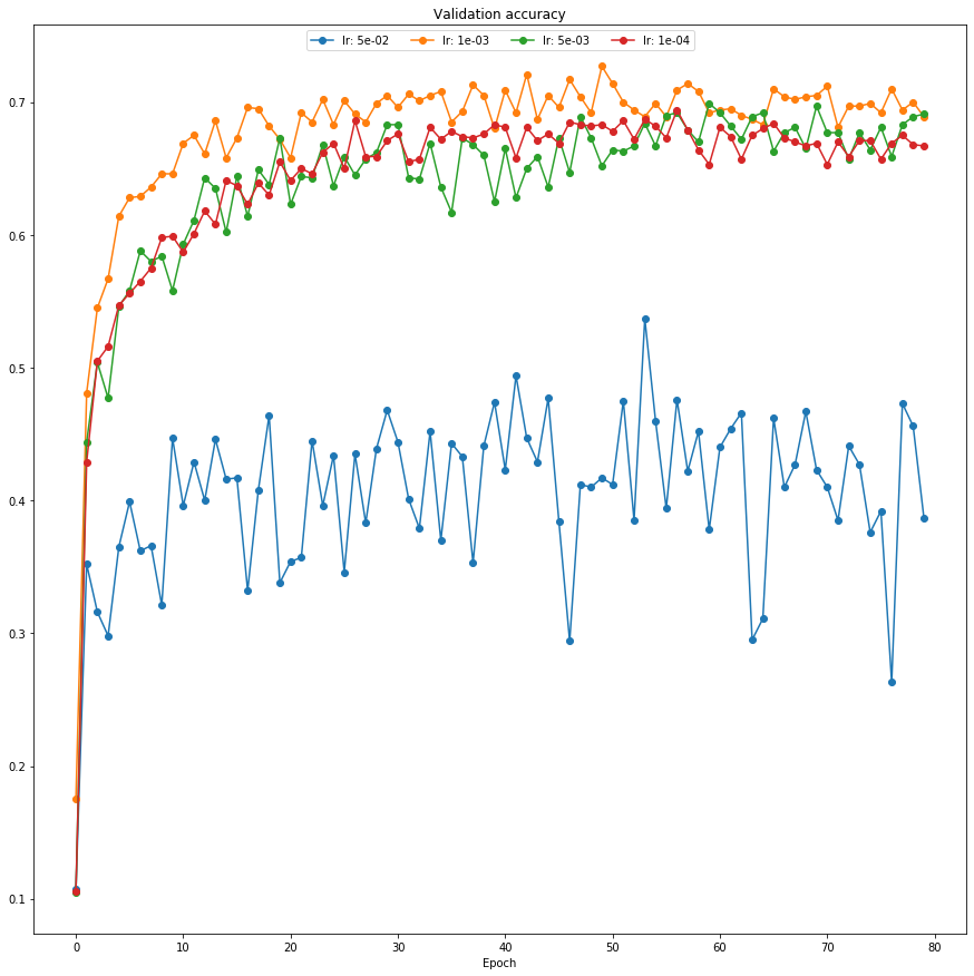
Test set – run this only once
Now that we’ve gotten a result we’re happy with, we test our final model on the test set (which you should store in best_model). Think about how this compares to your validation set accuracy.
best_model = model
check_accuracy_part34(loader_test, best_model)
Checking accuracy on test set
Got 6620 / 10000 correct (66.20)