CIFAR-10 k-Nearest Neighbor Classifier
Self Guided study of the course notes1 for cs231n: Convolutional Neural Networks for Visual Recognition provided Stanford University. Included in this page are references to the classes and function calls developed by Stanford university and others2 who have worked through this course material. The complete implementation of the k-NN classifier has been exported as a final Markdown file and can be found in the Jupyter Notebooks section of this site.
In this section, we will implement the k-Nearest Neighbor algorithm, (k-NN), for use in a an image classification system. The system will then be implemented and tested against the CIFAR-103 4 dataset. The objective of this implementation is to accurately assign a single label to each of the images within the test set based on a set of predetermined categories.
- Loading the CIFAR-10 dataset
- k-Nearest Neighbor Algorithm
- Cross-validation to find the best k
- Refereneces
Loading the CIFAR-10 Dataset
The CIFAR-10 dataset is a labeled subset of 60,000 (32x32) color images which were collected by Alex Krizhevsky, Vinod Nair, and Geoffrey Hinto. The images are categorized within 1 of 10 separate classifications, with 6,000 images per class. The complete dataset contains 50,000 training images along with 10,000 test images. The test images were created using “exactly 1,000 randomly-selected images from each class”. Figure 1 below shows a subsample of 7 images from each class along with the corresponding labels for each class.
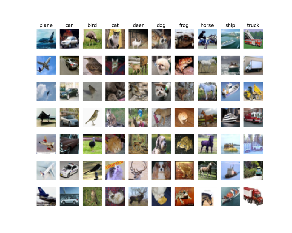
Figure 1: Samples from the CIFAR-10 Dataset
The first step in this process was to simply load the raw CIFAR-10 data into python. A quick preview of the loaded data is shown in Figure 1 above.
# Load the raw CIFAR-10 data.
cifar10_dir = 'cs231n/datasets/cifar-10-batches-py'
# Training images, training labels, test images, test labels
X_train, y_train, X_test, y_test = load_CIFAR10(cifar10_dir)

# View some basic details of the CIFAR-10 data
print('Training data shape: ', X_train.shape)
print('Training labels shape: ', y_train.shape)
print('Test data shape: ', X_test.shape)
print('Test labels shape: ', y_test.shape)
Training data shape:  (50000, 32, 32, 3)
Training labels shape:  (50000,)
Test data shape:  (10000, 32, 32, 3)
Test labels shape:  (10000,)
Looking at the above output, we can see that we’ve loaded all 50,000 (32x32) training images, the 10,000 (32x32) test images, and the corresponding labels for each set. To help make the development process more efficient, a subsample of 5,000 training images and 500 test images will be created, (python processing code not shown).
...
print(X_train.shape, X_test.shape)
(5000, 3072) (500, 3072)
k-Nearest Neighbor Algorithm
The k-nearest neighbors algorithm is a classification method in which the classification of a sample object is determined based on its k-nearest neighbors, where k is a user defined parameter and the classification of the surrounding neighbors is known. It assumes that objects close to each other are similar to each other. The k-NN is defined as a non-parametric method in which the algorithm makes no assumptions about the underlying data sets. It is also an instance-based learning algorithm, (i.e. a lazy algorithm), in which the training data is not used to make any generalizations on the test data set. This means that the “training” step in a k-NN is very short, leaving the majority of the data processing to the classification step. Consequently, this makes the k-NN an inherently poor choice for large data sets. However, the algorithm is simple, easy to implement, and versatile, which makes it a great choice for understanding basic concepts in image classification.
Calculating L2 (Euclidean) Distance
Knowing that the classification, (i.e. label) of an image can be predicted based on its k-nearest neighbors, a system for comparing images is then required. One method for doing so is to calculate the Euclidean distance, (L2 Distance), between all images within both the test and training data sets. The L2 distance is the “straight-line” distance between any two points and can be calculated as follows.
Using the function above, the L2 distance between any two images is accomplished by first squaring the results of the pixel-wise difference between the two images. The values of the output matrix are then summed together, from which a final square root is taken. The final scalar value obtained describes the L2 distance between the two input images. Doing this against all images in both the test and training data sets, a final matrix is created which documents the L2 distance between all images.
Two-loop Implementation
Converting the algorithm into a python function, the natural assumption is to think that the L2 Distance for all images is calculated by iterating through all images within both data sets, (i.e. a for loop with a nested for loop).
        num_test = X.shape[0]
        num_train = self.X_train.shape[0]
        dists = np.zeros((num_test, num_train))
        for i in range(num_test):
            for j in range(num_train):
                #####################################################################
                # Compute the l2 distance between the ith test point and the jth    #
                # training point, and store the result in dists[i, j].              #
                #####################################################################
                dists[i,j] = (((self.X_train[j,:] - X[i,:])**2).sum())**0.5
        return dists
The output of this process, (Figure 2) contains a plot of the L2 distance matrix for all test and training images within the subsample data set. Note that in a previous step, a subsample of the complete data set was obtained. This included 5000 training images, (expressed below along the X-axis) and 500 test images, (expressed on the Y-axis). The axis values capture the index location of each image within its respective data set while the L2 distance is defined by the intensity value displayed in the graph. Dark points represent a lower L2 distance value while lighter points represent a higher L2 distance.
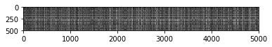
Figure 2: L2 (Euclidean) Distance Matrix
With the L2 distance matrix available, the label of an image within the test set can be assigned based on a “majority vote” of its k-nearest neighbors. From Figure 2 above, we can see that the L2 distance between test Image[0] and every training image is located along a single horizontal axis. By sorting these values, the k lowest values can then be used to make a prediction on the classification of Image[0].
# Now implement the function predict_labels with a value k=1
y_test_pred = classifier.predict_labels(dists, k=1)
...
for i in range(dists.shape[0])
    label_index = dists[i,:].argsort()
    closest_y = self.y_train[label_index[0:k]]
    y_pred[i] = np.bincount(closest_y).argmax()

return y_pred
...
# Show results of prediction
num_correct = np.sum(y_test_pred == y_test)
accuracy = float(num_correct) / num_test
print('Got %d / %d correct => accuracy: %f' % (num_correct, num_test, accuracy))
Doing this for all images within the test dataset, we’re able to predict the labels of the test images with an accuracy of 27.4%.
Got 137 / 500 correct => accuracy: 0.274000
Adjusting the number of neighbors to k=5, we obtain a slightly higher accuracy with our classifier.
y_test_pred = classifier.predict_labels(dists, k=5)
num_correct = np.sum(y_test_pred == y_test)
accuracy = float(num_correct) / num_test
print('Got %d / %d correct => accuracy: %f' % (num_correct, num_test, accuracy))
Got 139 / 500 correct => accuracy: 0.278000
No-Loop Implementation
Although the two loop version utilized some python vector processing techniques, the whole process can be optimized using a fully-vectorized process. The end result will eliminate both of the for loops an decrease processing time. This is accomplished through python vectorized processing.
num_test = X.shape[0]
num_train = self.X_train.shape[0]
dists = np.zeros((num_test, num_train))
dists = np.sqrt((X**2).sum(axis=1)[:, np.newaxis] + (self.X_train**2).sum(axis=1) - 2 * X.dot(self.X_train.T))
Comparing the processing time for each method, we see a significant increase in performance with the fully-vectorized version.
Two loop version: 25.233699 seconds
No loop version: 0.335277 seconds
Cross Validation to find the best k-value
As was shown in the two loop implementation, it is possible to increase the accuracy of our predictions by increasing the number of neighbors k. However, there is a single value of k that will return the highest degree of accuracy in our prediction. The best value of k can be determined through a cross validation process where the training data is split into n equal sets, or folds. Using the folds, we then run the k-NN algorithm for each value of k against [n-1] folds, leaving the last fold as a validation set. For the example below, the values k were limited to 10 choices.
num_folds = 5
k_choices = [1, 3, 5, 8, 10, 12, 15, 20, 50, 100]

X_train_folds = []
y_train_folds = []
################################################################################
# Split up the training data into folds. After splitting, X_train_folds and    #
# y_train_folds should each be lists of length num_folds, where                #
# y_train_folds[i] is the label vector for the points in X_train_folds[i].     #
################################################################################

X_train_folds = np.array_split(X_train, num_folds)
Y_train_folds = np.array_split(y_train, num_folds)

# A dictionary holding the accuracies for different values of k
k_to_accuracies = {}


################################################################################
# Perform k-fold cross validation to find the best value of k. For each        #
# possible value of k, run the k-nearest-neighbor algorithm num_folds times,   #
# where in each case you use all but one of the folds as training data and the #
# last fold as a validation set. Store the accuracies for all fold and all     #
# values of k in the k_to_accuracies dictionary.                               #
################################################################################

for k in k_choices:
    k_to_accuracies[k] = []

for k in k_choices:
    print('k=%d' % k)
    for j in range(num_folds):
        # Use all but one folds as our crossval training set
        X_train_crossval = np.vstack(X_train_folds[0:j] + X_train_folds[j+1:])
        # Use the last fold as our crossval test set
        X_test_crossval = X_train_folds[j]

        y_train_crossval = np.hstack(Y_train_folds[0:j]+Y_train_folds[j+1:])
        y_test_crossval = Y_train_folds[j]

        # Train the k-NN Classifier using the crossval training set
        classifier.train(X_train_crossval, y_train_crossval)

        # Use the trained classifer to compute the distance of our crossval test set
        dists_crossval = classifier.compute_distances_no_loops(X_test_crossval)

        y_test_pred = classifier.predict_labels(dists_crossval, k)
        num_correct = np.sum(y_test_pred == y_test_crossval)
        accuracy = float(num_correct) / num_test

        k_to_accuracies[k].append(accuracy)
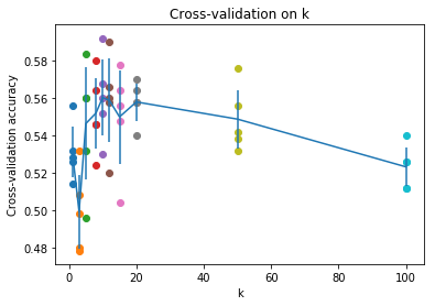
Figure 3: Cross-Validation Results
Using the Cross-Validation results above, it’s clear that the optimum value of k is 10. Running the k-NN one last time with k=10, we obtain the following results.
Got 141 / 500 correct => accuracy: 0.282000
Although the k-NN was useful for introducing some key concepts in image classification, it came with the following disadvantages:
- The classifier must store all of the training data for later use when trying to make predictions. Considering the size of both the training and test sets, this approach requires large amount of data and leads to issues with data storage. In terms of scalability, the data storage issue is amplified, becoming more problematic, as the data set grows.
- Ideally, the training portion of the classification system would be the most data intensive. This then implies that the prediction phase would be relatively quick. Conversely, with the k-NN, the training portion is relatively quick, while the prediction phase is the most data intensive.
References
-
CS231n Stanford University (2015, Aug).Convolutional Neural Networks for Visual Recognition [Web log post]. Retrieved from http://cs231n.stanford.edu/ ↩
-
Miranda, L. J. (2017, Feb 11).Implementing a multiclass support-vector machine [Web log post]. Retrieved from https://ljvmiranda921.github.io/notebook/2017/02/11/multiclass-svm/ ↩
-
Krizhevsky, A., Nair, V., and Hinton, G. (2009). CIFAR-10 (Canadian Institute for Advanced Research) [Web log post]. Retrieved from https://www.cs.toronto.edu/~kriz/cifar.html ↩
-
Krizhevsky, A., 2009. Learning Multiple Layers of Features from Tiny Images ↩