Multiclass Support Vector Machine (SVM)
Self Guided study of the course notes1 for cs231n: Convolutional Neural Networks for Visual Recognition provided through Stanford University. Included in this page are references to the classes and function calls developed by Stanford university and others2 who have worked through this course material. The complete implementation of the SVM classifier has been exported as a final Markdown file and can be found in the Jupyter Notebooks section of this site.
In this section, we continue the task of image classification on the CIFAR-103 4 labeled dataset. In this approach we’ll implement the Support Vector Machine, (SVM), a linear classification, supervised learning algorithm that works to identify the optimal hyperplane for linearly separable patterns.The final output of the model is a class identity. The SVM uses a linear function which assumes a boundary exists that separates one class boundary from another. The primary goal of the SVM is to efficiently find the boundary which separates one class from another. In this implementation, we will utilize a linear score function to compute a class score for the input data set. The output score can then be used within a loss function to better determine the success of the linear score function. Stochastic Gradient Descent will then be utilized as the optimization algorithm to minimize the loss obtained by the loss function.
- Loading the CIFAR-10 dataset
- Data Pre-Processing
- Linear Classification
- Hyperparameter Tuning and Cross Validation
- Refereneces
Loading the CIFAR-10 Dataset
Similar to the knn-implementation, the first step in this process is to load the raw CIFAR-10 data into python. A quick preview of the loaded data is shown in Figure 1 below.
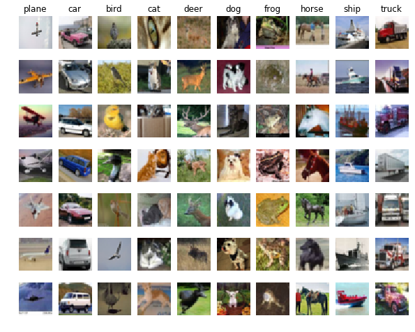
Figure 1: Samples from the CIFAR-10 Dataset
# Load the raw CIFAR-10 data.
cifar10_dir = 'cs231n/datasets/cifar-10-batches-py'
# Training images, training labels, test images, test labels
X_train, y_train, X_test, y_test = load_CIFAR10(cifar10_dir)

# View some details of the CIFAR-10 data
print('Training data shape: ', X_train.shape)
print('Training labels shape: ', y_train.shape)
print('Test data shape: ', X_test.shape)
print('Test labels shape: ', y_test.shape)
Training data shape:  (50000, 32, 32, 3)
Training labels shape:  (50000,)
Test data shape:  (10000, 32, 32, 3)
Test labels shape:  (10000,)
Data Pre-Processing
Prior to training the model, the data must be partitioning accordingly. From the 50,000 images within the training data, 49,000 images will be grouped as the official training set while the remaining 1,000 images will be designated as a validation set. The validation set will be used to tune the learning rate and regularization strength. From the 10,000 images within the test data set, a subsample of 1,000 images will be used to evaluate the accuracy of the SVM. A separate development data set of 500 randomly selected images will be created for use during development.
# Split the data into 4 data sets, training, validation, test, and dev.
num_training = 49000
num_validation = 1000
num_test = 1000
num_dev = 500

# Create validation set based on last 1000 images from training set
mask = range(num_training, num_training + num_validation)
X_val = X_train[mask]
y_val = y_train[mask]

# Create training set based on first 49000 images within original training set
mask = range(num_training)
X_train = X_train[mask]
y_train = y_train[mask]

# Create development subset of 500 random sampled images from training set
mask = np.random.choice(num_training, num_dev, replace=False)
X_dev = X_train[mask]
y_dev = y_train[mask]

# Create test set from first 1000 images within original test set
mask = range(num_test)
X_test = X_test[mask]
y_test = y_test[mask]

print('Train data shape: ', X_train.shape)
print('Train labels shape: ', y_train.shape)
print('Validation data shape: ', X_val.shape)
print('Validation labels shape: ', y_val.shape)
print('Test data shape: ', X_test.shape)
print('Test labels shape: ', y_test.shape)
Train data shape:  (49000, 32, 32, 3)
Train labels shape:  (49000,)
Validation data shape:  (1000, 32, 32, 3)
Validation labels shape:  (1000,)
Test data shape:  (1000, 32, 32, 3)
Test labels shape:  (1000,)
Each image is then reshaped from a 3-dimensional, (32 x 32) matrix, into a single 3072 element array. The end result for each image set is a 2-D ( x 3072) array of images.
# Preprocessing: reshape the image data into rows
X_train = np.reshape(X_train, (X_train.shape[0], -1))
X_val = np.reshape(X_val, (X_val.shape[0], -1))
X_test = np.reshape(X_test, (X_test.shape[0], -1))
X_dev = np.reshape(X_dev, (X_dev.shape[0], -1))

print('Training data shape: ', X_train.shape)
print('Validation data shape: ', X_val.shape)
print('Test data shape: ', X_test.shape)
print('Dev data shape: ', X_dev.shape)
Training data shape:  (49000, 3072)
Validation data shape:  (1000, 3072)
Test data shape:  (1000, 3072)
Dev data shape:  (500, 3072)
Finally, we’ll normalize the dataset by subtracting the mean of the training data from each of the datasets outlined above. Subtracting the dataset mean centers the data and helps to keep the feature dataset within a similar range of each other which is beneficial when processing the gradient.
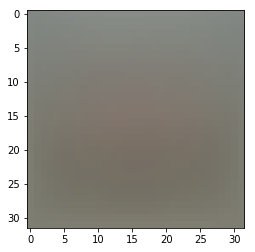
Figure 2: Mean of the Training Data Set
Linear Classification
Implementation of a linear classifier can be thought of as a template matching algorithm where each class within an input weight matrix is iteratively adjusted to create a best fit template for the class it represents. The adjusted weights are then used in the score function when trying to make a prediction against an unknown input image. In our case this would be the test image dataset. The output of this process is a final score value for each class which specifies how closely the input image maps to the corresponding class.
Linear Score Function
The SVM is implemented by first computing the linear score function of the data set. The linear score function uses the dot product of the input training data, , and the randomly generated weight matrix with a shape of x . Note that the length of the first dimension matches the total number of (pixels + 1) within each image. The additional pixel, (which was also added to each image set) is the addition of the bias vector which influences the output score without directly interacting with the input training data.
# generate a random SVM weight matrix of small numbers
W = np.random.randn(3073, 10) * 0.0001
From these parameters we arrive at the following function.
At this point we can make a few observations about the linear score function. The dot product of the two matrices results in an array of 10 separate scores for each image. As was mentioned previously, the weights were randomly generated, which suggests that we have the ability to adjust these input values. As we train the model, the goal is to adjust such that the output score for the correct class is significantly higher than the output scores of the incorrect classes. This step of fine-tunning the model will be accomplished by calculating the loss of the linear score function and minimizing our loss through stochastic gradient descent. The end result from this iterative process is a final weight matrix which can be used to map an input image to the appropriate class label .
Loss Function
Simply put, the loss function quantifies the accuracy of the linear score function by comparing the score of the correct class against the scores of the incorrect classes. Using the linear score function, we calculate the score for the class , as well as the score of the correct class for image . We then determine weather or not the score of the correct class is greater than the incorrect class by some fixed margin . Doing this across the entire data set we end up with a final loss value, sometimes refereed to as a cost score.
Taking the average loss and applying a regularization penalty of weighted by the hyperparameter , we obtain the following.
Stochastic Gradient Descent
Having defined the loss function, we now want to find the values of which minimize the loss function. Starting with a random set of weights, we can iteratively refine the values to produce a slightly better score than previously defined. This optimization process is accomplished most affectively by calculating the gradient of the loss function with respect to the input weights.
Stepping through the derivation, we first re-write the the loss function in terms of the input parameters, and .
We then expand the gradient to evaluate the partial derivative with respect to both the current class and the ground truth class .
Looking at initially for a single observation, for all classes where , we can see that the partial derivatives evaluates to when and zero otherwise.
The final expression for can then be re-written using the indicator function .
Evaluating for a single observation, we’re now looking at the gradient with respect to the correct class . As noted previously, the ideal is that the score of the correct class be greater than the score of the incorrect class by some fixed margin . This becomes a summation of all the classes where the score did not met the margin and contributed to the loss.
The final python implementation using a nested for loop is shown below.
    dW = np.zeros(W.shape) # initialize the gradient as zero

    # compute the loss and the gradient
    num_classes = W.shape[1]
    num_train = X.shape[0]
    loss = 0.0
    for i in range(num_train):
        scores = X[i].dot(W)
        correct_class_score = scores[y[i]]
        for j in range(num_classes):
            if j == y[i]:
                continue
            margin = scores[j] - correct_class_score + 1 # note delta = 1
            if margin > 0:
                loss += margin
                dW[:,y[i]] -= X[i,:]
                dW[:,j] += X[i,:]

    # Divide all over training examples
    dW /= num_train
    # Add regularization
    dW += reg * W

    # Right now the loss is a sum over all training examples, but we want it
    # to be an average instead so we divide by num_train.
    loss /= num_train

    # Add regularization to the loss.
    loss += reg * np.sum(W * W)


    return loss, dW
We can optimize this code further as a completely vectorized implementation.
    loss = 0.0
    dW = np.zeros(W.shape) # initialize the gradient as zero

    # compute the loss and the gradient
    num_classes = W.shape[1]
    num_train = X.shape[0]

    loss = 0.0
    # Calculate the scores matrix
    scores_v = X.dot(W)
    # Calculate the correct score index
    # Create list containing two 1D arrays
    # 1st array = index of images Xi
    # 2nd array = index for correct class value Yi
    correct_score_index = [np.arange(scores_v.shape[0]), y]
    # Select correct score from score matrix using [Xi, Yi]
    correct_class_score_v = scores_v[correct_score_index]
    # Calculate margin, utilize np.newaxis to broadcast correct class value
    # across 10 columns
    margin = scores_v - correct_class_score_v[:, np.newaxis] + 1
    # Set values less than zero equal to zero
    margin[margin < 0] = 0
    # Account for condition where j == Yi
    margin[correct_score_index] = 0
    # sum total loss
    loss = margin.sum()
    # take the average loss
    loss /= num_train
    # apply regularization
    loss += 0.5 * reg * np.sum(W * W)

    # This mask can flag the examples in which their margin is greater than 0
    X_mask = np.zeros(margin.shape)
    X_mask[margin > 0] = 1

    # As usual, we count the number of these examples where margin > 0
    count = np.sum(X_mask,axis=1)
    X_mask[np.arange(num_train),y] = -count

    dW = X.T.dot(X_mask)

    # Divide the gradient all over the number of training examples
    dW /= num_train

    # Regularize
    dW += reg*W


    return loss, dW
Having defined an efficient expressions for the loss and gradient, we can train the model by adjusting the input weights using the gradient. However, rather than calculating the gradient for every input image , this will be done iteratively over several sub samples of the data set, (i.e. Stochastic Gradient Descent). With each sample iteration, a small adjustment will be made to the weight matrix using a predefined learning rate and the gradient calculation.
    def train(self, X, y, learning_rate=1e-3, reg=1e-5, num_iters=100,
              batch_size=200, verbose=False):
        """
        Train this linear classifier using stochastic gradient descent.

        Inputs:
        - X: A numpy array of shape (N, D) containing training data; there are N
          training samples each of dimension D.
        - y: A numpy array of shape (N,) containing training labels; y[i] = c
          means that X[i] has label 0 <= c < C for C classes.
        - learning_rate: (float) learning rate for optimization.
        - reg: (float) regularization strength.
        - num_iters: (integer) number of steps to take when optimizing
        - batch_size: (integer) number of training examples to use at each step.
        - verbose: (boolean) If true, print progress during optimization.

        Outputs:
        A list containing the value of the loss function at each training iteration.
        """
        num_train, dim = X.shape
        num_classes = np.max(y) + 1 # assume y takes values 0...K-1 where K is number of classes
        if self.W is None:
            # lazily initialize W
            self.W = 0.001 * np.random.randn(dim, num_classes)

        # Run stochastic gradient descent to optimize W
        loss_history = []
        for it in range(num_iters):
            X_batch = None
            y_batch = None

            i_range = np.random.choice(np.arange(X.shape[0]), batch_size)
            X_batch = X[i_range, :]
            y_batch = y[i_range]

            # evaluate loss and gradient
            loss, grad = self.loss(X_batch, y_batch, reg)
            loss_history.append(loss)

            # perform parameter update
            # Update the weights using the gradient and the learning rate

            self.W += -learning_rate * grad

            # *****END OF YOUR CODE (DO NOT DELETE/MODIFY THIS LINE)*****

            if verbose and it % 100 == 0:
                print('iteration %d / %d: loss %f' % (it, num_iters, loss))

        return loss_history
Using the following input parameters when training the SVM, the loss converges to an approximate value of 5.
svm.train(X_train, y_train, learning_rate=1e-7, reg=2.5e4,
                      num_iters=1500, batch_size=200, verbose=True)
iteration 0 / 1500: loss 411.229123
iteration 100 / 1500: loss 242.353926
iteration 200 / 1500: loss 147.521380
iteration 300 / 1500: loss 90.800391
iteration 400 / 1500: loss 56.806474
iteration 500 / 1500: loss 36.503065
iteration 600 / 1500: loss 23.774250
iteration 700 / 1500: loss 15.723157
iteration 800 / 1500: loss 11.630423
iteration 900 / 1500: loss 9.050186
iteration 1000 / 1500: loss 7.439663
iteration 1100 / 1500: loss 6.954062
iteration 1200 / 1500: loss 5.243393
iteration 1300 / 1500: loss 5.179514
iteration 1400 / 1500: loss 5.546934
Plotting the results of the training model.
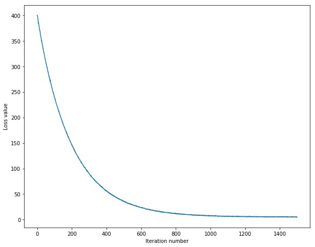
Figure 3: Training the SVM through Stochastic Gradient Descent
We can now evaluate the performance of the model against the training set and validation set. Calculating the linear score function using the trained parameters , we take the max value for each class to identify the predicted class.
y_pred = np.argmax(X.dot(self.W), 1)
Comparing these results against the actual labels, we obtain an accuracy of ~ 38%.
training accuracy: 0.382776
validation accuracy: 0.395000
Hyperparameter Tuning and Cross Validation
Finally, we’ll use the validation set to tune the regularization strength and learning rate hyperparameters. Using the following combination of inputs, we’ll train an SVM using the training set and evaluate the accuracy on both the training and validation set. The most accurate results can be used to identify the optimum combination of hyperparameters.
learning_rates = [1e-8, 1e-7, 2e-7]
regularization_strengths = [1e4, 2e4, 3e4, 4e4, 5e4, 6e4, 7e4, 8e4, 1e5]
Looking at a few of the results.
...
lr 1.000000e-07 reg 3.000000e+04 train accuracy: 0.380224 val accuracy: 0.385000
lr 1.000000e-07 reg 4.000000e+04 train accuracy: 0.374163 val accuracy: 0.381000
lr 1.000000e-07 reg 5.000000e+04 train accuracy: 0.370714 val accuracy: 0.389000
lr 1.000000e-07 reg 6.000000e+04 train accuracy: 0.364571 val accuracy: 0.379000
lr 1.000000e-07 reg 7.000000e+04 train accuracy: 0.365204 val accuracy: 0.365000
Plotting the results for the entire set on a logarithmic scale, we see that the most accurate results were obtained when using a learning rate of x and a regularization strength of x. Using these parameters, we were able to get an accuracy of 37.1% on the training set and an accuracy of 38.9% on the validation set.
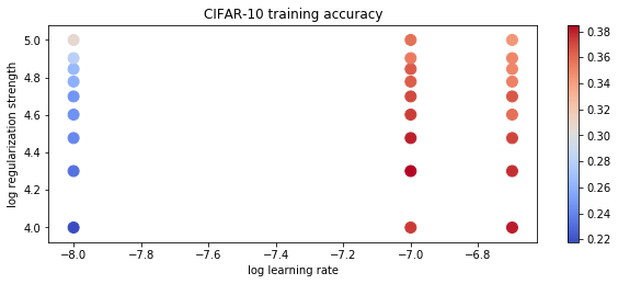
Figure 4: CIFAR-10 Prediction Accuracy on Training Set
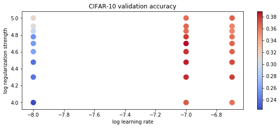
Figure 5: CIFAR-10 Prediction Accuracy on Validation Set
Visualizing the learning weights for each class, we can start to see some similarities between each of the learned templates. For instance, the animal classes bird and horse have significantly more green in the template. This is most likely due to the fact that these images are often taken outside, (in nature), which tends to have more green. As a result, this model would likely be biased towards classifying an image as a bird or a horse when encountered with an image with a lot of green.
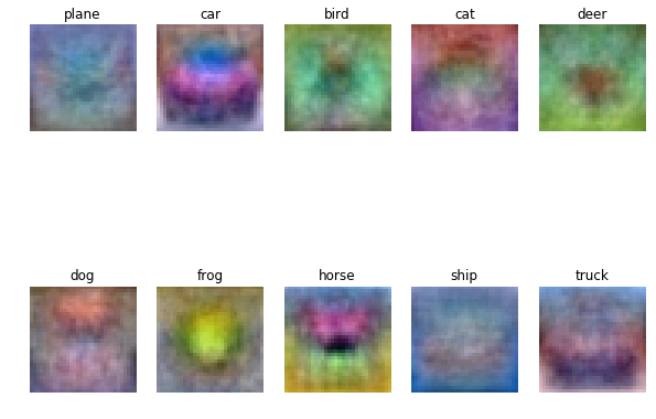
Figure 6: Visualization of learned weights
Unlike the knn-implementation previously discussed, the training data is discarded once the trained parameters are learned. When making a prediction, the paramaters are used in a single dot product operation which is computationally inexpensive. However, this implemenation of the SVM has its limitation when it comes to over generalization. As was shown in figure 6, the templates for various classes have a tendancy to be categorized based on a dominant color within the background, (as opposed to the object itself).
References
-
CS231n Stanford University (2015, Aug).Convolutional Neural Networks for Visual Recognition [Web log post]. Retrieved from http://cs231n.stanford.edu/ ↩
-
Miranda, L. J. (2017, Feb 11).Implementing a multiclass support-vector machine [Web log post]. Retrieved from https://ljvmiranda921.github.io/notebook/2017/02/11/multiclass-svm/ ↩
-
Krizhevsky, A., Nair, V., and Hinton, G. (2009). CIFAR-10 (Canadian Institute for Advanced Research) [Web log post]. Retrieved from https://www.cs.toronto.edu/~kriz/cifar.html ↩
-
Krizhevsky, A., 2009. Learning Multiple Layers of Features from Tiny Images ↩