Building a Two Layer Neural Network
Self Guided study of the course notes1 for cs231n: Convolutional Neural Networks for Visual Recognition provided through Stanford University. Included in this page are references to the classes and function calls developed by Stanford university and others, [Miranda2, Voss3], who have worked through this course material. The complete implementation of the Two-Layer Neural Network has been exported as a final Markdown file and can be found in the Jupyter Notebooks section of this site.
In this post, we’ll work through the steps and theory for developing a Two Layer Neural Network. The initial model will be generated and tested using a toy data set. Once we’re able to obtain ideal testing and validation results using the toy dataset, we’ll extend the application of the Two Layer Neural Network onto the CIFAR-104 5 labeled dataset for image classification.
- Neural Network Architecture
- Development (Toy Model)
- Development (CIFAR-10)
- Hyperparameter Tuning
- Refereneces
Neural Network Architecture
Data Organization and Computation
In the previous post we developed an image classification model using a SVM classifier, supervised learning algorithm that works to identify the optimal hyperplane for linearly separable patterns. The SVM uses a linear “scoring” function, which assumes a boundary exists that separates one class boundary from another. The scoring function was computed using the dot product of the input training data set and the randomly generated weight matrix . In this example, was a set of images, (i.e. row vectors) containing 3072 pixels each plus an additional bias dimension , for a final shape of x . The weight matrix in this example consisted of 10 column vectors of size 3072 randomly generated weights, (plus a bias ). The final matrix of shape x represented each possible classification within the data set, providing us with a set of parameters that could then be learned through Stochastic Gradient Descent, (SGD).
For this implementation of a neural network, we’ll utilize the softmax scoring function as our linear classifier and extend the scoring process across two separate layers consisting of a hidden layer and final output layer. As a general example, we might generate two weight matrices, of shape x and of shape x , where the larger matrix will learn to identify larger features in the data set while the smaller weight matrix will learn to identify smaller, detail specific features. The final score is then computed as follows.
In the above expression, the function, otherwise know as a ReLU activation function, works as a non-linearity which provides a separation between the two weight matrices and . This separation in turn is what allows us to train each set of parameters through SGD. This implementation of a neural network effectively executes a series of linear mapping functions which are then tied together through activation functions, (i.e. non-linear functions). A simple visualization of this network is shown in Figure 1.
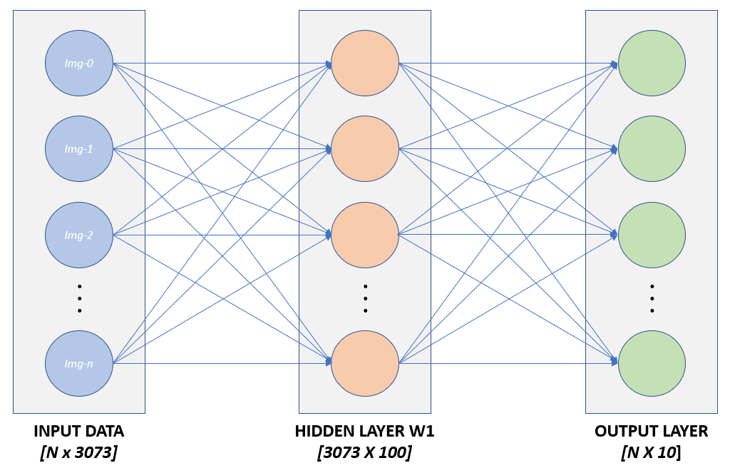
Figure 1: Graphical Representation of a Two Layer Neural Network
Note that the “first layer” of an N-Layer neural network starts after the input layer. Figure 1 shows an input layer and a 2 layer neural network, comprised of a hidden layer and an output layer. Also omitted from the graphic in figure one are details regarding the activation function which is calculated as part of the hidden layer.
Development (Toy Model)
Having a basic foundation for the architecture of the network, we begin development using a toy data set of arbitrary data and the associated labels . Looking at the input data set , we see that we have a total of 5, 4-dimensional data points in the x matrix.
print(X)
[[ 16.24345364  -6.11756414  -5.28171752 -10.72968622]
 [  8.65407629 -23.01538697  17.44811764  -7.61206901]
 [  3.19039096  -2.49370375  14.62107937 -20.60140709]
 [ -3.22417204  -3.84054355  11.33769442 -10.99891267]
 [ -1.72428208  -8.77858418   0.42213747   5.82815214]]

print(y)
[0 1 2 2 1]
While creating this data set, we simultaneously generate an instance of our two-layer neural network.
net = TwoLayerNet(input_size, hidden_size, num_classes, std=1e-1)
Although we’re currently developing a neural network to classify the “toy data set” noted above, the same class instance will be utilized below when applied to the CIFAR-10 dataset. As such, the input parameters to the class instance will be discussed with respect to both the toy data set and the CIFAR-10 data set. This will hopefully provide additional context to the class design, input parameters, and how the data sets relate to one another, specifically the input data and weight matrices and . The input parameters for this class instance are defined as follows:
- input_size: Dimension D
- Captures the second dimension of the training data set, (i.e. number of columns)
- Toy Data Set: D = 4
- CIFAR-10 Set: D = 3072
- hidden_size:
- Specifies the size of the second dimension within the first weight matrix
- Toy Data Set: 10
- CIFAR-10 Set: Range between 50 and 300 (discussed below)
- Specifies the size of the second dimension within the first weight matrix
- num_classes:
- Total number of classes in final output
- Toy Data Set: 5
- CIFAR-10 Set: 10
- Total number of classes in final output
Weight Initialization
Using the input parameters defined above, the class instantiation generates weight and bias parameters internally. both weight matrices are initialized to small random values which are further scaled according to the input parameter . Bias terms are initialized to zero, however these values are updated at a later step while training the model. Note that the random seed is set to a value of zero which produces the same set of random variables with every instance. This allows for repeatable testing and trouble shooting during development.
self.params = {}
np.random.seed(0)
self.params['W1'] = std * np.random.randn(input_size, hidden_size)
self.params['b1'] = np.zeros(hidden_size)
self.params['W2'] = std * np.random.randn(hidden_size, output_size)
self.params['b2'] = np.zeros(output_size)
Forward Pass Computation
The forward pass defines the steps in which we execute linear mapping, activation functions, apply regularization, and calculate the loss of the new scoring function. Conversely, during back propagation, (discussed below), we compute the gradient by propagating backwards through the forward pass computation using the chain rule. Using the toy data set defined above, the forward pass computation starts by calculating the linear score function of the input data set and the first weight matrix . The activation function is then applied which thresholds all activations below zero to a value of zero. The results of this output are then passed into the next linear mapping function to generate the final score output for each class.
# First layer linear score function
h1 = X.dot(W1) + b1

# First layer activation function
a1 = np.maximum(0, h1)

# Output Layer score function
scores = a1.dot(W2) + b2
Activation Function
Using a biological neuron as a model, the activation function is used to model the firing rate of a neuron. In the biological model, each neuron receives input information from its dendrites and produces output information along the axon which is then carried to other neurons. We model the input information as a multiplication of the input data and the learned weights which represent the synaptic strength of the neuron. If the linear combination of this input information exceeds a certain threshold, than the neuron will “fire”, sending and output signal along the axon to other neurons. We model this functionality using the Rectified Linear Unit, (ReLU), function which computes the function . Similar to the biological neuron, the input provided to the ReLU function is the output from the linear scoring function , which corresponds to the input data and learned weights. From here the ReLU, (i.e. activation function) will than output the linear scoring function if the value of said score exceeds a certain threshold, (i.e. zero). Other commonly used activation functions include the sigmoid function, Tanh, ReLU, Leaky ReLU and Maxout, all of which are discussed in great detail under the Neural Networks Part 1 - Commonly Used Activation Functions section of the course notes. For our purposes, we’ll stick with the Rectified Linear Unit, (ReLU).
Loss Function
Using the Minimal Neural Network Case Study1 section from the course notes as a reference for computing the loss, we can implement the loss function for a Softmax classifier. The loss of the class scores using the loss function is defined as:
As mentioned in the same section, “the full Softmax classifier loss is then defined as the average cross-entropy loss over the training examples and the regularization”1:
exp_scores = np.exp(scores)
probs = exp_scores / np.sum(exp_scores, axis=1, keepdims=True)

corect_logprobs = -np.log(probs[range(N), y])
data_loss = np.sum(corect_logprobs) / N
reg_loss = 0.5 * reg * np.sum(W1 * W1) + 0.5 * reg * np.sum(W2 * W2)
loss = data_loss + reg_loss
Regularization
As shown in the code snippet above, regularization is applied to the loss function to avoid over fitting. Over fitting occurs when the model learns to many of the details within the data set, including undesirable information such as noise. Regularization allows us to prevent over fitting by causing the network to generalize information affectively thus improving overall performance. In this section, we implement L2 regularization, which has the affect of penalizing the squared magnitude of the weight matrices . L2 regularization is also known as weight decay since it has the effect of causing the weights to decay towards zero. Note that the regularization strength is one of the hyperparameters we’ll analyze at a later step as part of hyperparameter optimization.
SGD Through Backpropogation
From the Minimal Neural Network Case Study1 in the course notes, we’re given the following expression along with the final evaluation for the gradient .
# compute gradient on scores
dscores = probs
dscores[range(N),y] -= 1
dscores /= N
With the gradient for the scores available, we can now backpropogate through the two layer network and calculate the gradient with respect to the weight and bias parameters. We can evaluate these expressions through dimension analysis and identification of various Patterns in backward flow1. As described in the course notes, the local gradient of a multiply gate has the property of multiplying the input parameters against the backpropogated gradient received from the “downstream” function. For example, given the following expression,
And given the gradient of the end function with respect to
The through backpropogation is derived as:
By intuition:
Extending this analysis to Gradients of vectorized operations1, we can apply the same logic and deduce the organization of the matrix multiplication by analysis of each matrices dimensions. The final implementation is given below.
# gradient for W2 and b2
grads['W2'] = np.dot(a1.T, dscores)
grads['b2'] = np.sum(dscores, axis=0)

# Backpropagate to h1
dh1 = np.dot(dscores, W2.T)

# Backpropagate ReLU non-linearity
dh1[a1 <= 0] = 0

#
grads['W1'] = np.dot(X.T, dh1)
grads['b1'] = np.sum(dh1, axis=0)

grads['W2'] += 2 * reg * W2
grads['W1'] += 2 * reg * W1
Parameter Updates
Having calculated the gradients, we can now perform a parameter optimization. For this implementation, we’ll stick with the “vanilla update” which updates the parameters along the negative gradient direction and scales the update according to the learning rate constant.
self.params['W1'] += -learning_rate * grads['W1']
self.params['b1'] += -learning_rate * grads['b1']
self.params['W2'] += -learning_rate * grads['W2']
self.params['b2'] += -learning_rate * grads['b2']
Training
Finally, we want to train and evaluate the performance of our two-layer neural network. We’ll first create an instance of the class object TwoLayerNet() and then provide the class instance with the toy data set and the hyperparameters “learning rate” and “regularization strength”.
net = init_toy_model()
stats = net.train(X, y, X, y,
            learning_rate=1e-1, reg=5e-6,
            num_iters=100, verbose=False)
Without speaking to the provided code in the train() function, the first task is to generate a mini batch of the training data. One of the reasons for doing this step is to avoid degradation of the model quality. The three contrasting types of gradient descent are Stochastic Gradient Descent, Batch Gradient Descent, and Mini-Batch Gradient Descent, (each of which having their own pros and cons). Stochastic gradient Descent updates the parameters after each example within the training data set. Batch Gradient Descent calculates the error for all training examples, (i.e. one training epoch) before updating the parameters. Mini-batch Gradient Descent attempts to combine the two methodologies by lumping the training data into mini-batches. Updates to the parameters are made after evaluating the error for each example within the mini-batch.
idx = np.random.choice(range(X.shape[0]), batch_size)
X_batch = X[idx]
y_batch = y[idx]
Sticking with the mini-batch implementation as noted by the assignment instructions, we then calculate the loss and gradient for the current batch and update the parameters as follows.
self.params['W1'] += -learning_rate * grads['W1']
self.params['b1'] += -learning_rate * grads['b1']
self.params['W2'] += -learning_rate * grads['W2']
self.params['b2'] += -learning_rate * grads['b2']
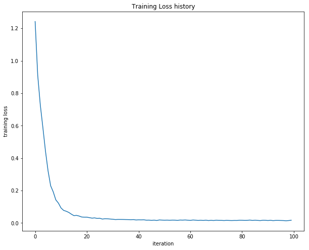
Figure 2: Training loss after each training iteration
Plotting these results, we can observe a decreasing training loss which converges around 0.017. From this, we can conclude that everything is working as expected. We can now begin test this implementation against the larger CIRFAR-10 data set.
Development (CIFAR-10)
Similar to the knn-implementation and SVM-Classifier, the first step in this process is to load the raw CIFAR-10 data into python. A quick preview of the loaded data is shown in Figure 4 below.
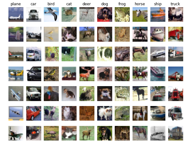
Figure 4: Samples from the CIFAR-10 Dataset
After data preprocessing, which includes zero averaging the data set and organizing each image into a single column vector, we end up with the following data sets. For clarity, the shape of each data set is noted.
X_train: Train data shape:  (49000, 3072)
y_train: Train labels shape:  (49000,)
X_val: Validation data shape:  (1000, 3072)
y_val: Validation labels shape:  (1000,)
X_test: Test data shape:  (1000, 3072)
y_test: Test labels shape:  (1000,)
# Normalize the data: subtract the mean image
mean_image = np.mean(X_train, axis=0)
X_train -= mean_image
X_val -= mean_image
X_test -= mean_image
With minimal effort, we can create a neural net class instance and train the network using the CIFAR-10 data set. Note that the train function calls the loss function internal which calculates the loss and gradients discussed above.
input_size = 32 * 32 * 3
hidden_size = 50
num_classes = 10
net = TwoLayerNet(input_size, hidden_size, num_classes)
print(net.params['W1'].shape)
# Train the network
stats = net.train(X_train, y_train, X_val, y_val,
            num_iters=1000, batch_size=200,
            learning_rate=1e-4, learning_rate_decay=0.95,
            reg=0.25, verbose=True)
Setting the verbose parameter equal to True, we can view the convergence of the loss function as we train the network. From this simple output, we see that the results are not favorable, converging at a value around 1.967. Moreover, testing the trained network against the validation data set, we receive an accuracy of 28.2%. Comparing these results to that of the SVM from the previous section, where we obtained an accuracy of 38.9%, we can conclude that the network is not performing optimally. This leads us to the task of debugging and hyper parameter tuning. In Figure 5, we visualiz the results of the learned parameters from this effort.
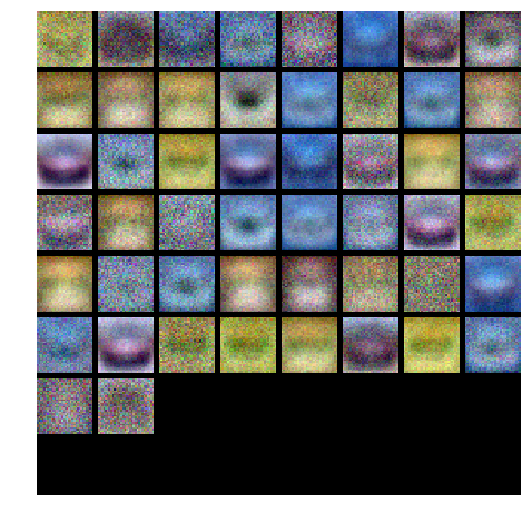
Figure 5: Learned Parameters
iteration 0 / 1000: loss 2.302976
iteration 100 / 1000: loss 2.302638
iteration 200 / 1000: loss 2.299256
iteration 300 / 1000: loss 2.270635
iteration 400 / 1000: loss 2.219117
iteration 500 / 1000: loss 2.141064
iteration 600 / 1000: loss 2.129066
iteration 700 / 1000: loss 2.047454
iteration 800 / 1000: loss 1.988162
iteration 900 / 1000: loss 1.967131

# Predict on the validation set
val_acc = (net.predict(X_val) == y_val).mean()
print('Validation accuracy: ', val_acc)

Validation accuracy:  0.282
Hyperparameter Tuning
As stated, we wish to optimize our network through hyper parameter tuning. By observation of Figure 6, the gap between the training accuracy and the validation accuracy remains low, which provides reassurance that we’re not over fitting. However, we can better understand the affects of regularization strength on the model by fine tunning the regularization strength. Another hyperparameter to analyze is the learning rate. Large learning rates have the tendency to result in unstable training, causing the model to converge rapidly to a suboptimal solution. Small leaning rates on the other hand risk getting stuck and fail to train the network. Finally, we’ll look at the total number of training iterations as well as how adjustments to the number of neurons in the hidden layer affect overall performance. Again, looking at Figure 6, the validation accuracy maintains an upward slope through training, suggesting that we simply haven’t provided the network with enough iterations. Referencing source code made available by Miranda2 and Voss3, the final implementation for hyperparameter tuning is shown below.
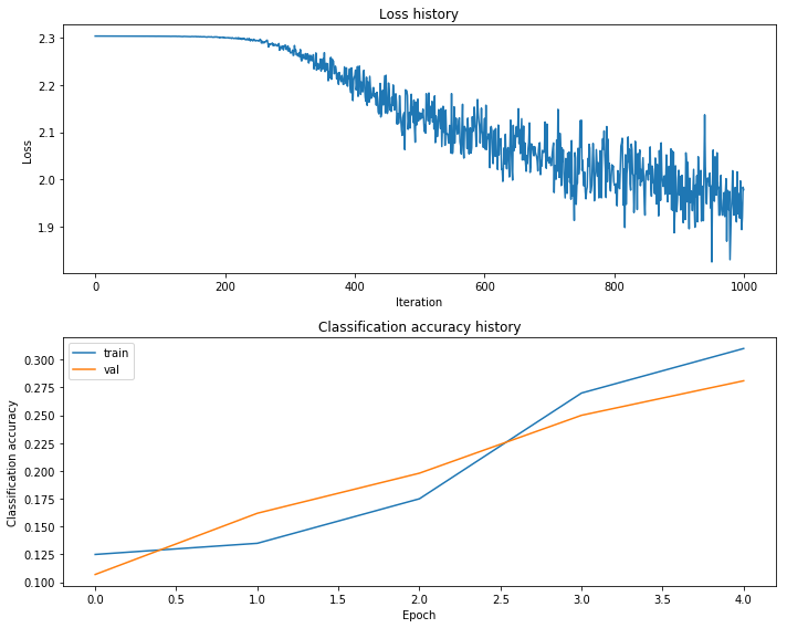
Figure 6: Training Results: Loss, Training Accuracy, & Validation Accuracy
best_net = None # store the best model into this

best_val = -1
best_stats = None
h = [100, 150, 200]
learning_rates = [1e-3, 1e-4, 1e-5]
regularization_strengths = [0.3, 0.4, 0.5]
results = {}
iters = 3000
for hidden_size in h:
    for lr in learning_rates:
        for rs in regularization_strengths:
            net = TwoLayerNet(input_size, hidden_size, num_classes)

            # Train the network
            stats = net.train(X_train, y_train, X_val, y_val,
                        num_iters=iters, batch_size=200,
                        learning_rate=lr, learning_rate_decay=0.95,
                        reg=rs, verbose=True)

            # Make predictions against training set
            train_pred = net.predict(X_train)
            # Get average training prediction accuracy
            train_acc = np.mean(y_train == y_train_pred)
            # Make predictions against validation set
            val_pred = net.predict(X_val)
            # Get average validation prediction accuracy
            val_acc = np.mean(y_val == val_pred)

            # Store results in dictionary using hyperparameters as key values
            results[(hidden_size, lr, rs)] = (hidden_size, train_acc, val_acc)

            # Update best validation accuracy if better results are obtained
            if val_acc > best_val:
                best_stats = stats
                best_val = val_acc
                best_net = net

# Print out results.
for h, lr, reg in sorted(results):
    hidden_size, train_accuracy, val_accuracy = results[(h, lr, reg)]
    print('h %s lr %e reg %e train accuracy: %f val accuracy: %f' % (
                h, lr, reg, train_accuracy, val_accuracy))

print('best validation accuracy achieved during cross-validation: %f' % best_val)
h 100 lr 1.000000e-05 reg 3.000000e-01 train accuracy: 0.620776 val accuracy: 0.194000
h 100 lr 1.000000e-05 reg 4.000000e-01 train accuracy: 0.620776 val accuracy: 0.194000
h 100 lr 1.000000e-05 reg 5.000000e-01 train accuracy: 0.620776 val accuracy: 0.194000
h 100 lr 1.000000e-04 reg 3.000000e-01 train accuracy: 0.620776 val accuracy: 0.391000
h 100 lr 1.000000e-04 reg 4.000000e-01 train accuracy: 0.620776 val accuracy: 0.390000
.
.
.
best validation accuracy achieved during cross-validation: 0.52000
Looking at the output results, (python print statements above), we obtain a validation accuracy of 52.0% acquired using the following parameters.
- Learning Rate: 1e-3
- Regularization Strength: 0.3
- Hidden Layer Size: 150
Plotting the training history for the net with the best validation accuracy, Figure 7, we’re able to see the loss history, training accuracy, and validation accuracy as we train the network. It is worth noting how the validation and training accuracies begin to diverge after approximately 2 epochs, suggesting that we may be overfitting the data beyond this point.
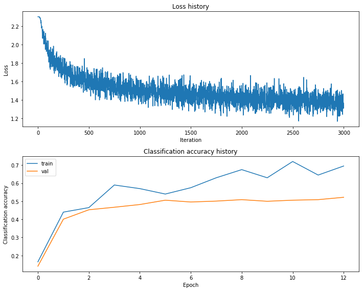
Figure 7: Training Results (After HyperParameter Tuning): Loss, Training Accuracy, & Validation Accuracy
Visualizing the weights of the learned parameters, Figure 8, we can start to see some details emerge in the learned weights.
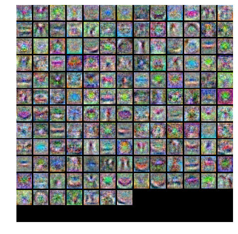
Figure 8: Visualization of Learned Parameters
Finally, we implement the model of learned weights using the test data set. From this step we we obtain a test accuracy of 52%.
test_acc = (best_net.predict(X_test) == y_test).mean()
print('Test accuracy: ', test_acc)

Test accuracy:  0.52
References
-
CS231n Stanford University (2015, Aug).Convolutional Neural Networks for Visual Recognition [Web log post]. Retrieved from http://cs231n.stanford.edu/ ↩ ↩2 ↩3 ↩4 ↩5 ↩6
-
Miranda, L. J. (2017, Feb 17). Implementing a two-layer neural network from scratch [Web log post]. Retrieved from https://ljvmiranda921.github.io/notebook/2017/02/17/artificial-neural-networks/ ↩ ↩2
-
Voss, C. (2015, Sep 22). CNN-Assignments [Web log post]. Retrieved from https://github.com/CatalinVoss/cnn-assignments/tree/master/assignment1 ↩ ↩2
-
Krizhevsky, A., Nair, V., and Hinton, G. (2009). CIFAR-10 (Canadian Institute for Advanced Research) [Web log post]. Retrieved from https://www.cs.toronto.edu/~kriz/cifar.html ↩
-
Krizhevsky, A., 2009. Learning Multiple Layers of Features from Tiny Images ↩